Hydrogen from radial shells to finite counts

3. Hydrogen: radial shells, normalization and finite profile control

3.1 The finite source and its exact radial data

Use one vertex per radial state $(n,\ell)$, $1\le n\le30$, $0\le\ell<n$: 465 vertices without a magnetic expansion. For $a_0=1$, the normalized radial functions are

$$R_{n\ell}(r)=\frac{2}{n^2}\sqrt{\frac{(n-\ell-1)!}{(n+\ell)!}}e^{-r/n}(2r/n)^\ell L_{n-\ell-1}^{2\ell+1}(2r/n).\tag{9}$$

For $|\ell-k|=1$ set $W_{n\ell,mk}=|\int_0^\infty R_{n\ell}(r)R_{mk}(r)r^3\,dr|^2$, and otherwise use zero. The Laplacian $L=D-W$ has 8,990 undirected edges including 435 same-shell links. The positive sector has dimension 464 and exposure 214,832. Its readout is

$$v_i=\log(1+\lambda_i/a),\qquad a=\lambda_{\min,+}(L).\tag{10}$$

This graph is distinct from the atomic Hamiltonian with energies $E_n=-1/(2n^2)$ and from the historical 78-state H12 graph. That construction omitted same-shell links and used absolute radial amplitudes with an $m=0$ angular factor. No H12 values enter here.

The finite Laguerre expansion of (9) reduces each integral to factorials and rational powers multiplied by the square root of a rational number. Squaring gives exact rational weights. The supplement regenerates all 8,990 weights, verifies exact same-shell fixtures and bounds the individual relative rounding errors of the stored binary64 graph by $u=2^{-53}$. This certifies scalar inputs, not all subsequent matrix operations.

3.2 An exact same-shell spectrum

For fixed $n$, Laguerre recurrence and orthogonality, or direct insertion of the terminating series, give

$$I_{n\ell,n,\ell+1}=-\frac32n\sqrt{n^2-(\ell+1)^2},\qquad w_{n,\ell}=\frac94n^2[n^2-(\ell+1)^2].\tag{11}$$

The radial integral has a negative sign, which disappears in the squared construction.

Proposition 3.1 (Same-shell modes). The path on $\ell=0,\ldots,n-1$ with weights (11) has eigenvalues

$$\lambda_{n,r}^{(0)}=\frac94n^2(2r)(2r+1),\qquad r=0,\ldots,n-1.\tag{12}$$

Proof. On nodes $j=0,\ldots,m$, the operator

$$\mathcal Af(j)=(j+1)(m-j)[f(j)-f(j+1)]+j(m-j+1)[f(j)-f(j-1)]$$

preserves polynomial degree and multiplies the leading term of $j^k$ by $k(k+1)$. The filtration triangularizes the $(m+1)$-dimensional operator with distinct eigenvalues $k(k+1)$, $0\le k\le m$. Reflection $j\mapsto m-j$ commutes with it. The degree-$k$ eigenpolynomial has parity $(-1)^k$ because its leading term does and its eigenspace is one-dimensional. Set $m=2n-1$ and keep the even sector. Pairing reflected sites gives the $n$-node half-path with a reflecting endpoint. The central edge contributes zero. Reversing the half-path order gives weights $n^2-(\ell+1)^2$. Thus $k=2r$, and the factor $9n^2/4$ proves (12).

The same-shell direct sum has 30 zero modes. Inter-shell edges lift 29 and retain the global constant. The lifted shell-constant directions belong in the original statistic. At cutoff 30 the same-shell edges carry about 76.77% of the weight, while the adjacent-shell graph retains 1,276 edges and about 97.92%. Those fractions organize the calculation, but do not bound sharp counts near a small minimum.

There is a continuum account for the disconnected raw shell levels. Under the triangular state count, $x=n/N$ and $y=r/n$ have limiting measure $2x\,dx\,dy$, and $\lambda^{(0)}/N^4\to9x^4y^2$. Hence $\sqrt{\lambda^{(0)}/N^4}/3$ has the law of a product of two independent uniforms with CDF $t(1-\log t)$. The corresponding independent raw log-difference density is $(|d|+2)e^{-|d|/2}/16$. This describes the raw disconnected spectrum, rather than the full finite minimum-normalized one.

3.3 Adjacent shells, the minimum and signed cancellation

Let $B$ retain edges with $|n-m|\le1$, and write

$$L=B+R_g+R_c,\tag{13}$$

where $R_g$ contains the omitted edges incident on $1s$, and $R_c$ the other omitted edges. Both are positive Laplacians. The small ground-incident weight supplies most of the minimum motion, while core edges supply material high-mode shifts. The normalization mechanism and bulk mechanism can be separated without discarding either.

On the constant complement choose the unit contrast between $1s$ and the uniform rest and complete it orthogonally. The minimum follows from the source, with no insertion of the observed target eigenvalue:

$$L_+=\begin{pmatrix}\alpha&\xi^*\\\xi&H\end{pmatrix},\qquad a=\alpha-\xi^*(H-aI)^{-1}\xi.\tag{14}$$

If $H\ge gI$ with $g>\alpha$, Rayleigh's principle gives $a\le\alpha$. Comparing to a $2\times2$ matrix with diagonal $(\alpha,g)$ and off-diagonal $\|\xi\|$ bounds it below. The right side of (14) decreases below $g$, so reversed endpoint evaluation and intersection provide successive valid enclosures. A source Cholesky floor and geometric resolvent series avoid a full rest-spectrum diagonalization. The original-coordinate residual estimate gives $[2.05903639204,2.05903672699]$ approximately, with independently evaluated rest floor above $17.1341$. The interval uses the declared residual and rounding model, not directed interval arithmetic.

The function $F(\lambda,a)=\log\log(1+\lambda/a)$ satisfies

$$dF=\eta(\lambda/a)(d\log\lambda-d\log a),\qquad \eta(x)=\frac{x}{(1+x)\log(1+x)}.\tag{15}$$

Since $\eta$ decreases, a moving minimum acts differently on low and high modes. A pair retains only the difference of their motions. Define the full, fixed-minimum baseline and own-minimum baseline vectors by $P_0=P(\lambda,a)$, $P_1=P(b,a)$ and $P_2=P(b,b_1)$. With $E_s=P_1-P_0$ and $E_a=P_2-P_1$, use the exact vector decomposition before taking norms:

$$P_2-P_0=(P_1-P_0)+(P_2-P_1).\tag{16}$$

The two RMS contributions are about $2.08828\times10^{-4}$ and $1.88192\times10^{-4}$. Their sum has RMS $6.05482\times10^{-5}$ and the cosine is about $-0.9588$. Positivity alone does not force cancellation: the ground-only and core-only interventions lose it. Common scaling $R=cB$ instead cancels exactly under (10).

The fixed 16-mode predictor retains mixing within each block. Diagonalize $B$ on the constant complement, with basis $V$ and eigenvalues $b_i$. Set $A=\operatorname{diag}(b)+V^*RV$ and use consecutive 16-mode projectors $P_j$:

$$D_{16}=\sum_j P_jAP_j.\tag{17}$$

Pool and sort block eigenvalues, replace the first by the independently derived $a$, and apply the original readout and windows. The omitted cross-block matrix is available for error control. Natural-case componentwise RMS error is about $2.86437\times10^{-5}$. The predicted total discrepancy $5.96993\times10^{-5}$ is close to the actual discrepancy, but agreement of magnitudes is weaker than agreement of coordinates. The baseline eigensolve and dense source transform remain required; no speed advantage follows.

Table 1. Source-reconstructed controls for $B+gR_g+cR_c$. Predicted, actual and error are RMS over 45 coordinates in units of $10^{-4}$: the predicted and actual uncorrected discrepancy and the componentwise prediction error. Cosine compares the actual $E_s,E_a$ in (16). These are known mathematical development controls.

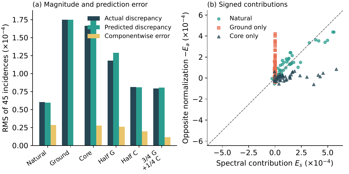
Figure 1. Hydrogen control calculations from all 45 coordinates. G and C denote ground and core remainders. Panel (a) separates discrepancy magnitude from componentwise prediction error. Each point in (b) is one coordinate of the spectral contribution against the opposite normalization contribution. The dashed line denotes exact cancellation. No sampling uncertainty or independent empirical observation is represented.

The six controls compare the predictor to direct source-graph validation. Ground-only has almost no spectral contribution (RMS $2.08\times10^{-6}$), with normalization contribution $1.75\times10^{-4}$. Core-only has spectral contribution $1.79\times10^{-4}$ and normalization contribution $3.18\times10^{-5}$. Natural mixing yields the smaller total discrepancy and cosine $-0.95878$. Mixed controls change the cancellation by changing the relative weights. Ground-only's zero predictor error concerns the 45 integer coordinates, not equality of its complete spectrum. The public code regenerates each minimum, all target and predictor coordinates, the signed terms, the table and the plot.

3.4 Signed shell self-energies and a radial convergence bound

Retain matrix blocks and ranks rather than tracking perturbative eigenvectors through crossings. For an orthogonal retained projector $P$, put $Q=I-P$. Write the source in the $B$ basis as $\left(\begin{smallmatrix}A_{PP}&C\\ C^*&H\end{smallmatrix}\right)$. For real $x$, the Schur matrix is

$$S(x)=A_{PP}-xI-C(H-xI)^{-1}C^*.\tag{18}$$

Congruence gives $n_-(A-xI)=n_-(H-xI)+n_-(S(x))$ where the exterior inverse exists. Negative exterior directions keep their signs. Replacing the virtual contributions by positive norms loses the cancellation.

Split the remainder by principal-shell lag: $R=R_2+R_3+R_{\rm far}$, with far lag at least four. Keep the full $C$ and $A_{PP}$. On the exterior space $Q\mathcal H$, with $Q$ as identity, use

$$D_0=Q(B+R_2+R_3-\sigma I)Q,\qquad E=QR_{\rm far}Q,\qquad G_0(x)=[D_0-(x-\sigma)I]^{-1}.$$

Theorem 3.2 (Signed exterior expansion). Suppose $\operatorname{dist}(0,\operatorname{spec}D_0)\ge g$, $|x-\sigma|\le r<g$, and $\|E\|\le\beta<d=g-r$. Put $\rho=\beta/d$. For every integer $m\ge0$,

$$(H-xI)^{-1}=\sum_{j=0}^m(-G_0E)^jG_0+R_m,\qquad \|R_m\|\le\frac{\rho^{m+1}}{d(1-\rho)}.\tag{19}$$

Every retained word is selfadjoint. Congruence by $C$ gives a two-sided Loewner bound on the self-energy error of size $\|C\|^2\rho^{m+1}/[d(1-\rho)]$. Exterior inertia is constant in the window and along the homotopy from zero to $E$.

Proof. The gap gives $\|G_0\|\le1/d$. Factor $H-xI=(D_0-(x-\sigma)I)(I+G_0E)$. Expand the last inverse geometrically. The remainder $(-G_0E)^{m+1}(I+G_0E)^{-1}G_0$ has the stated bound. Each word $(G_0E)^jG_0=G_0EG_0\cdots EG_0$ equals its adjoint without commutativity. The true inverse and finite sum are selfadjoint, turning the norm bound into a two-sided scalar Loewner bound. Finally, $\|tE\|<d$ for $0\le t\le1$ excludes zero eigenvalues throughout the homotopy and window, proving constant inertia.

Lag-two and lag-three interference remain in $D_0$ and the full coupling. Their quadratic and cross-term signs are not universal. An independent rational fixture with indefinite $D_0=\operatorname{diag}(-2,3)$ and noncommuting positive $E$ verifies the ordering and remainder for degrees zero through seven. Endpoint rank brackets give ordered eigenvalue intervals without assuming monotonicity of the truncated noncommuting polynomial.

The radial bound comes before matrix compression. Let $u_{n\ell}=rR_{n\ell}$ be normalized in $L^2(dr)$. Its squared moment is

$$M_{n\ell}=\|ru_{n\ell}\|^2=\frac{n^2}{2}[5n^2+1-3\ell(\ell+1)].\tag{20}$$

For each admitted adjacent angular channel $k$, the functions $u_{mk}$ are orthonormal. Apply Bessel's inequality to the disjoint union of finite lags at most three, finite far states and the selected exterior states $m=31,32,33$. For $\nu(\ell)$ admitted channels,

$$d_{\rm far}(n,\ell)\le\nu(\ell)M_{n\ell}-d_{\le3}(n,\ell) -\sum_{\substack{m=31,32,33\\ k\ \mathrm{admitted}}}W_{n\ell,mk}.\tag{21}$$

Only channels admitted by the graph enter, so there is no upward channel from $\ell=29$. No continuum completeness is assumed. Within each channel the subtracted vectors are orthogonal to the finite far subset; continuum and higher-shell contributions leave nonnegative slack.

For nonnegative graph weights, $\|L_{\rm far}\|\le 2\max_i d_{\rm far}(i)$ from $|z_i-z_j|^2\le2(|z_i|^2+|z_j|^2)$. Orthogonal compression does not increase the bound. The coarse moment-minus-retained value $1.620289\times10^6$ fails contraction in three of four required sectors because of radial weight beyond the cutoff. Subtracting the three exterior shells gives the verified upper bound

$$\beta=33507.79904140163.\tag{22}$$

Exact Fraction arithmetic evaluates 2,789 retained and 2,697 external weights and saves each row budget. Regenerating 8,990 original edges verifies the rounding premise and all 465 stored far-row inequalities. Under $|\widehat W-W|\le uW$, division by $1-u$ transfers the budget to the stored graph. The floating upper is compared to that rational bound. These are exact scalar and edge certificates; exterior gaps, inverse residuals, products and inertia remain numerical matrix evaluations.

3.5 Returning the bound to all original counts

The six formerly unresolved windows use 53 partner ranks. Four sectors of dimensions $96,96,96,48$ have radial expansion ratios approximately $0.12183,0.08096,0.06291,0.01893$. Degrees $5,4,4,3$ with widened endpoints pass 106 rank checks after charging assembly, gap, inverse-substitution, product and eigen-residual allowances. The narrower failed endpoint widening remains a diagnostic. The successful return keeps actual far-edge entries in the correction words, rather than predicting from only a few scalar moments.

Given positive spectral intervals $[\ell_i,u_i]$ and common minimum interval $[a_-,a_+]$, monotonicity gives

$$\log(1+\ell_i/a_+)\le v_i\le \log(1+u_i/a_-).$$

Each pair uses the same minimum in both entries. Equation (15) gives monotonicity of its ratio in $a$ at fixed spectral endpoints, so common endpoints suffice, with the minimum mode anchored exactly at $\log 2$. Guaranteed and possible memberships enclose each integer count. Mixed low/high membership can instead use the raw threshold $a[(1+\lambda_i/a)^q-1]$ and source inertia. Reversing a below-one window requires reciprocal endpoints, not a fresh symmetric tolerance.

The final calculation recovers all 45 H30 coordinates numerically and agrees with independent target diagonalization. SUM totals are $23495,7800,3895$ and UNION totals $21892,7800,3895$, agreeing only where windows do not overlap. Counts for $\sqrt2$ are $5433,1792,894$; for $\log2$, $4858,1621,821$. The complete generated counts appear in Appendix C, and the supplement retains all signed predictor errors.

Partner discovery takes 1,856 cached Schur queries beyond setup and 106 endpoint checks. Earlier mixed-count work used thousands of full-size inertia evaluations. The exact budget uses 5,486 retained-plus-exterior calls, including 2,697 exterior acquisitions, plus 8,990 for stored-edge verification. Actual far-coupling words and exterior-gap work remain essential. The signed correction converges and reaches the finite observable; a cheaper cutoff-uniform amplitude law is still open.

3.6 Cutoff concentration and the informative finite tail

Theorem 3.3 (Concentration of the native comparison statistic). For full and adjacent-shell squared-radial graphs at cutoff $N$, the incidence of every fixed window in (6) at each of the three tolerances tends to zero as $N\to\infty$ under its own minimum-normalized readout. Their 45-coordinate RMS difference tends to zero.

Proof. Put $q=N(N+1)/2$. Both graphs dominate the same-shell direct sum. Equation (20) bounds maximum degree by $5N^4$, hence $\lambda_{\max}\le10N^4$. The $1s$ degree is at most three, so its centered Rayleigh vector gives $a\le C_N=3q/(q-1)$. A positive mode is bad if $\lambda<N^{7/2}$. Min-max and Proposition 3.1 bound their number by the $N$ shell zero modes plus pairs with $9n^2r^2<N^{7/2}$. Summing $\min(n,O(N^{7/4}/n))$ over shells gives a bad fraction $O(N^{-1/4}\log N)+O(N^{-1})$.

For two good modes, the largest possible ratio is bounded by

$$Q_N=\frac{\log(1+10N^4/C_N)}{\log(1+N^{7/2}/C_N)}\longrightarrow\frac87.$$

For fixed rates it increases with $a$ by the decreasing elasticity in (15). Each above-one window has lower endpoint at least $0.97\sqrt2>8/7$; each below-one upper endpoint is below $7/8$. Eventually no good/good pair qualifies. For $b$ bad modes out of $m=q-1$, each incidence and UNION are bounded by

$$1-\frac{(m-b)(m-b-1)}{m(m-1)}\longrightarrow0.$$

The coordinate-vector difference tends to zero.

The growing bulk is compressed toward ratio one. This limit does not give the small H30 discrepancy: the explicit finite bounds are loose. The informative tail, common minimum and signed correction remain essential. A cutoff limit is a weaker discriminator than reconstructing the actual finite amplitudes and their response to source interventions.