# From Source Structure to Spectral Profiles: Generation Mechanisms and Observable Readouts in the Canonical Spectral-Curvature Framework
Generation Mechanisms and Observable Readouts in the Canonical Spectral-Curvature Framework
Jeremy Rodgers · 2026-11-03
DOI: https://doi.org/10.5281/zenodo.23912447
## Three ways to generate a spectral profile
**Three different source constructions generate the measured spectral profiles.** Radial-shell coupling and signed corrections recover all 45 hydrogen counts. Gaussian exchange transfers a spatial preparation law to a limiting ratio distribution. The angular and outgoing radial equations jointly recover the 540 Kerr labels. The same observable can compare these distinct mechanisms without identifying their microscopic laws.
## 1. The source-selection problem
A spectral comparison comes at the end of a chain of choices. A source law supplies an operator or boundary problem, preparation selects accessible states, a readout transforms the retained spectrum, and a pair statistic pools the values. Similarity at the last stage can reflect structure at any of these stages. An explanation must start from specified source data and reach the original statistic with control of what each transformation does.
The [spectral-ratio investigation](/source-readout/spectral-ratios) records recurrence, discrimination against conditional references, robustness and diagnostic limits for the hydrogen radial graph, gravitational Kerr damping and image-derived Gaussian graphs. The [Canonical Spectral-Curvature Field](/source-readout/cscf) gives the common-carrier architecture and locates the finite ratio observable in the modular calculus. The present development supplies generation mechanisms and quantitative controls, reaching the retained finite profiles from radial rules, spatial preparation and outgoing boundary conditions.
Hydrogen has an explicit finite source. Normalized Coulomb radial functions determine every squared edge weight rationally, same-shell chains have a closed spectrum, and omitted shells affect the minimum and bulk differently. In Gaussian spatial networks, the Laplacian spectrum follows the distribution of kernel mass at prepared sites. In Kerr, the open boundary problem generates frequency and damping together. Its poles cannot generally be represented by a nondecreasing frequency symbol on a damping-only carrier.
The evidence is layered. Finite identities and conditional theorems are proved here. Exact rational arithmetic checks scalar radial budgets, stored edges and independent finite fixtures. Matrix inverses, gaps, eigenvalues, inertia and resonance continuation use disclosed numerical arithmetic. Same-code repeatability, independent eigensolvers and separately formulated fixtures answer different questions. None is an atomic or image-formation experiment.
## 2. Realizations, readouts and retained information
### 2.1 The mathematical interface to CSCF and Shadow Theory
$$
\begin{gathered}
\text{source law and preparation}\
\longrightarrow\text{metric, carrier or boundary poles}\
\longrightarrow\text{retained readout}\
\longrightarrow\text{pair profile}.
\end{gathered}\tag{1}
$$
Each arrow requires data. Geometry alone supplies neither mobility nor a physical clock, energy form or detector. In the [source–readout foundations](/source-readout), descent is target-relative: exact recovery requires a target constant on each readout fibre. Geometric realization requires compatible metric, domain and boundary data. Exact projected dynamics retain unresolved preparation and memory unless an invariance condition removes them. These constraints organize the arrows in [(1)](/source-readout/spectral-profiles/01-sources-and-readouts#equation-1), while the Coulomb, Gaussian and Kerr laws supply their mechanisms.
In a finite CSCF realization, a declared Hermitian nonnegative form $Q$ has representative $K\ge0$ on the Hilbert carrier. With nonnegative symmetric graph weights $W$,
$$
Q(z)=z^*Lz=\sum_{i
$$
S_t=e^{-tK},\qquad C=h(K),\qquad U_s=e^{-isC}.\tag{3}
$$
The faces share a carrier within a realization. Different domains can have different operators and dimensions. A physical identification of $K$ needs energy and mobility, or an equivalent kinetic derivation; a physical identification of $C$ needs a reactive law in the same modal coordinates.
For example, linearize $\dot q=-M(q)\nabla F(q)$ at a stationary point $q_*$, with $M_*>0$ and $H=\operatorname{Hess}F\ge0$. The coordinate $y=M_*^{-1/2}(q-q_*)$ obeys
$$
\dot y=-Ky,\qquad K=M_*^{1/2}HM_*^{1/2}.\tag{4}
$$
The product of mobility and curvature has inverse-time units; curvature alone need not. A reversible population generator $Q_M$ with stationary probability $\pi$ instead gives $K=-D_\pi^{1/2}Q_MD_\pi^{-1/2}$. Detailed balance makes it selfadjoint with stationary vector $\sqrt\pi$. These metric distinctions determine the dipole-bath construction below.
### 2.2 The original finite observable
Retain labelled positive readouts $v_1,\ldots,v_m$, $m\ge2$, including multiplicities. Given the eligible set $B_r$ with nonzero exposure, define
$$
E=\{(i,j):i\ne j,\ v_i/v_j\in B_r\},\qquad N_R=|E|.\tag{5}
$$
The fifteen coordinates, in their original order, are
$$
(\phi,\phi^{-1},\phi^2,\sqrt2,\sqrt3,\sqrt5,\pi,\pi/2,\pi/10,e,e^{-1},\log 2,j_{0,1},3/13,1/7),
\tag{6}
$$
where $\phi=(1+\sqrt5)/2$ and $j_{0,1}$ is the first positive zero of $J_0$. For each $\epsilon\in\{0.03,0.01,0.005\}$ and center $c_k$,
$$
h_k=\sum_{(i,j)\in E}\mathbf 1_{[c_k(1-\epsilon),c_k(1+\epsilon)]}(v_i/v_j),\qquad
p_k=h_k/N_R.\tag{7}
$$
The windows are closed. Hydrogen and spatial networks retain all $m(m-1)$ ordered nonself pairs. Kerr uses $B_r=(0.05,5)$, which is open. SUM adds the counts and includes overlap multiplicity; UNION counts each pair in the union once.
Set $u_i=\log v_i$. The complete nonself log-ratio measure is
$$
\nu=\frac1{m(m-1)}\sum_{i\ne j}\delta_{u_i-u_j}
=\frac{m}{m-1}\mu*\check\mu-\frac1{m-1}\delta_0,\qquad
\mu=\frac1m\sum_i\delta_{u_i}.\tag{8}
$$
Reflection $u\mapsto-u$ gives $\check\mu$. Self-pair removal is labelled, so equal values from distinct modes still contribute. On the Hilbert–Schmidt space of the positive retained operator $V$, the normalized state $\rho=V/\operatorname{tr}V$ has eigenvalues $v_i/\sum_jv_j$. Its modular action $X\mapsto\rho X\rho^{-1}$ has eigenvalues $v_i/v_j$, with logarithm $[\log V,\cdot]$. This gives an exact spectral-calculus interpretation. It does not establish a quantum preparation of an image graph or calibrate a physical clock for the log-difference conjugate variable.
The centers in [(6)](/source-readout/spectral-profiles/01-sources-and-readouts#equation-6) remain comparison coordinates. The prior paired-library fraction $0.2339$ failed the frozen $0.05$ criterion. Generating the vector supplies no new evidence for exclusive library privilege. The 45 coordinates, a full ratio measure, scalar spectrum, operator readout and calibrated temporal response are distinct inputs to an inverse problem.
## Hydrogen from radial shells to finite counts
## 3. Hydrogen: radial shells, normalization and finite profile control
### 3.1 The finite source and its exact radial data
Use one vertex per radial state $(n,\ell)$, $1\le n\le30$, $0\le\ell
$$
R_{n\ell}(r)=\frac{2}{n^2}\sqrt{\frac{(n-\ell-1)!}{(n+\ell)!}}e^{-r/n}(2r/n)^\ell L_{n-\ell-1}^{2\ell+1}(2r/n).\tag{9}
$$
For $|\ell-k|=1$ set $W_{n\ell,mk}=|\int_0^\infty R_{n\ell}(r)R_{mk}(r)r^3\,dr|^2$, and otherwise use zero. The Laplacian $L=D-W$ has 8,990 undirected edges including 435 same-shell links. The positive sector has dimension 464 and exposure 214,832. Its readout is
$$
v_i=\log(1+\lambda_i/a),\qquad a=\lambda_{\min,+}(L).\tag{10}
$$
This graph is distinct from the atomic Hamiltonian with energies $E_n=-1/(2n^2)$ and from the historical 78-state H12 graph. That construction omitted same-shell links and used absolute radial amplitudes with an $m=0$ angular factor. No H12 values enter here.
The finite Laguerre expansion of [(9)](/source-readout/spectral-profiles/02-radial-shells#equation-9) reduces each integral to factorials and rational powers multiplied by the square root of a rational number. Squaring gives exact rational weights. The supplement regenerates all 8,990 weights, verifies exact same-shell fixtures and bounds the individual relative rounding errors of the stored binary64 graph by $u=2^{-53}$. This certifies scalar inputs, not all subsequent matrix operations.
### 3.2 An exact same-shell spectrum
For fixed $n$, Laguerre recurrence and orthogonality, or direct insertion of the terminating series, give
$$
I_{n\ell,n,\ell+1}=-\frac32n\sqrt{n^2-(\ell+1)^2},\qquad
w_{n,\ell}=\frac94n^2[n^2-(\ell+1)^2].\tag{11}
$$
The radial integral has a negative sign, which disappears in the squared construction.
**Proposition 3.1 (Same-shell modes).** The path on $\ell=0,\ldots,n-1$ with weights [(11)](/source-readout/spectral-profiles/02-radial-shells#equation-11) has eigenvalues
$$
\lambda_{n,r}^{(0)}=\frac94n^2(2r)(2r+1),\qquad r=0,\ldots,n-1.\tag{12}
$$
**Proof.** On nodes $j=0,\ldots,m$, the operator
$$
\mathcal Af(j)=(j+1)(m-j)[f(j)-f(j+1)]+j(m-j+1)[f(j)-f(j-1)]
$$
preserves polynomial degree and multiplies the leading term of $j^k$ by $k(k+1)$. The filtration triangularizes the $(m+1)$-dimensional operator with distinct eigenvalues $k(k+1)$, $0\le k\le m$. Reflection $j\mapsto m-j$ commutes with it. The degree-$k$ eigenpolynomial has parity $(-1)^k$ because its leading term does and its eigenspace is one-dimensional. Set $m=2n-1$ and keep the even sector. Pairing reflected sites gives the $n$-node half-path with a reflecting endpoint. The central edge contributes zero. Reversing the half-path order gives weights $n^2-(\ell+1)^2$. Thus $k=2r$, and the factor $9n^2/4$ proves [(12)](/source-readout/spectral-profiles/02-radial-shells#equation-12).
The same-shell direct sum has 30 zero modes. Inter-shell edges lift 29 and retain the global constant. The lifted shell-constant directions belong in the original statistic. At cutoff 30 the same-shell edges carry about 76.77% of the weight, while the adjacent-shell graph retains 1,276 edges and about 97.92%. Those fractions organize the calculation, but do not bound sharp counts near a small minimum.
There is a continuum account for the disconnected raw shell levels. Under the triangular state count, $x=n/N$ and $y=r/n$ have limiting measure $2x\,dx\,dy$, and $\lambda^{(0)}/N^4\to9x^4y^2$. Hence $\sqrt{\lambda^{(0)}/N^4}/3$ has the law of a product of two independent uniforms with CDF $t(1-\log t)$. The corresponding independent raw log-difference density is $(|d|+2)e^{-|d|/2}/16$. This describes the raw disconnected spectrum, rather than the full finite minimum-normalized one.
### 3.3 Adjacent shells, the minimum and signed cancellation
Let $B$ retain edges with $|n-m|\le1$, and write
$$
L=B+R_g+R_c,\tag{13}
$$
where $R_g$ contains the omitted edges incident on $1s$, and $R_c$ the other omitted edges. Both are positive Laplacians. The small ground-incident weight supplies most of the minimum motion, while core edges supply material high-mode shifts. The normalization mechanism and bulk mechanism can be separated without discarding either.
On the constant complement choose the unit contrast between $1s$ and the uniform rest and complete it orthogonally. The minimum follows from the source, with no insertion of the observed target eigenvalue:
$$
L_+=\begin{pmatrix}\alpha&\xi^*\\\xi&H\end{pmatrix},\qquad
a=\alpha-\xi^*(H-aI)^{-1}\xi.\tag{14}
$$
If $H\ge gI$ with $g>\alpha$, Rayleigh's principle gives $a\le\alpha$. Comparing to a $2\times2$ matrix with diagonal $(\alpha,g)$ and off-diagonal $\|\xi\|$ bounds it below. The right side of [(14)](/source-readout/spectral-profiles/02-radial-shells#equation-14) decreases below $g$, so reversed endpoint evaluation and intersection provide successive valid enclosures. A source Cholesky floor and geometric resolvent series avoid a full rest-spectrum diagonalization. The original-coordinate residual estimate gives $[2.05903639204,2.05903672699]$ approximately, with independently evaluated rest floor above $17.1341$. The interval uses the declared residual and rounding model, not directed interval arithmetic.
The function $F(\lambda,a)=\log\log(1+\lambda/a)$ satisfies
$$
dF=\eta(\lambda/a)(d\log\lambda-d\log a),\qquad
\eta(x)=\frac{x}{(1+x)\log(1+x)}.\tag{15}
$$
Since $\eta$ decreases, a moving minimum acts differently on low and high modes. A pair retains only the difference of their motions. Define the full, fixed-minimum baseline and own-minimum baseline vectors by $P_0=P(\lambda,a)$, $P_1=P(b,a)$ and $P_2=P(b,b_1)$. With $E_s=P_1-P_0$ and $E_a=P_2-P_1$, use the exact vector decomposition before taking norms:
$$
P_2-P_0=(P_1-P_0)+(P_2-P_1).\tag{16}
$$
The two RMS contributions are about $2.08828\times10^{-4}$ and $1.88192\times10^{-4}$. Their sum has RMS $6.05482\times10^{-5}$ and the cosine is about $-0.9588$. Positivity alone does not force cancellation: the ground-only and core-only interventions lose it. Common scaling $R=cB$ instead cancels exactly under [(10)](/source-readout/spectral-profiles/02-radial-shells#equation-10).
The fixed 16-mode predictor retains mixing within each block. Diagonalize $B$ on the constant complement, with basis $V$ and eigenvalues $b_i$. Set $A=\operatorname{diag}(b)+V^*RV$ and use consecutive 16-mode projectors $P_j$:
$$
D_{16}=\sum_j P_jAP_j.\tag{17}
$$
Pool and sort block eigenvalues, replace the first by the independently derived $a$, and apply the original readout and windows. The omitted cross-block matrix is available for error control. Natural-case componentwise RMS error is about $2.86437\times10^{-5}$. The predicted total discrepancy $5.96993\times10^{-5}$ is close to the actual discrepancy, but agreement of magnitudes is weaker than agreement of coordinates. The baseline eigensolve and dense source transform remain required; no speed advantage follows.
**Table 1. Source-reconstructed controls for $B+gR_g+cR_c$.** Predicted, actual and error are RMS over 45 coordinates in units of $10^{-4}$: the predicted and actual uncorrected discrepancy and the componentwise prediction error. Cosine compares the actual $E_s,E_a$ in [(16)](/source-readout/spectral-profiles/02-radial-shells#equation-16). These are known mathematical development controls.
| Control | $g$ | $c$ | Predicted | Actual | Error | Cosine |
| --- | ---: | ---: | ---: | ---: | ---: | ---: |
| Natural | 1 | 1 | 0.59699 | 0.60548 | 0.28644 | -0.95878 |
| Ground only | 1 | 0 | 1.75233 | 1.75233 | 0.00000 | 0.06870 |
| Core only | 0 | 1 | 1.78978 | 1.66763 | 0.28041 | -0.45157 |
| Half ground | 0.5 | 1 | 1.28992 | 1.18160 | 0.26203 | -0.88356 |
| Half core | 1 | 0.5 | 0.81043 | 0.81514 | 0.19810 | -0.94639 |
| $3R_g/4+R_c/4$ | 0.75 | 0.25 | 0.80785 | 0.79587 | 0.11673 | -0.90226 |
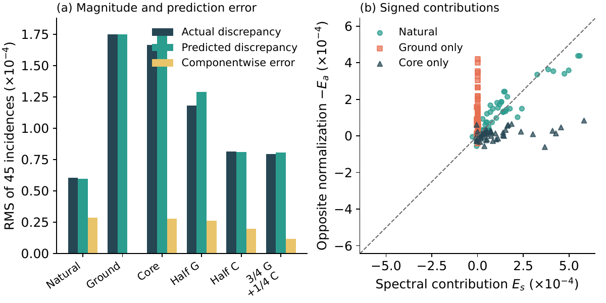
**Figure 1.** Hydrogen control calculations from all 45 coordinates. G and C denote ground and core remainders. Panel (a) separates discrepancy magnitude from componentwise prediction error. Each point in (b) is one coordinate of the spectral contribution against the opposite normalization contribution. The dashed line denotes exact cancellation. No sampling uncertainty or independent empirical observation is represented.
The six controls compare the predictor to direct source-graph validation. Ground-only has almost no spectral contribution (RMS $2.08\times10^{-6}$), with normalization contribution $1.75\times10^{-4}$. Core-only has spectral contribution $1.79\times10^{-4}$ and normalization contribution $3.18\times10^{-5}$. Natural mixing yields the smaller total discrepancy and cosine $-0.95878$. Mixed controls change the cancellation by changing the relative weights. Ground-only's zero predictor error concerns the 45 integer coordinates, not equality of its complete spectrum. The public code regenerates each minimum, all target and predictor coordinates, the signed terms, the table and the plot.
### 3.4 Signed shell self-energies and a radial convergence bound
Retain matrix blocks and ranks rather than tracking perturbative eigenvectors through crossings. For an orthogonal retained projector $P$, put $Q=I-P$. Write the source in the $B$ basis as $\left(\begin{smallmatrix}A_{PP}&C\\ C^*&H\end{smallmatrix}\right)$. For real $x$, the Schur matrix is
$$
S(x)=A_{PP}-xI-C(H-xI)^{-1}C^*.\tag{18}
$$
Congruence gives $n_-(A-xI)=n_-(H-xI)+n_-(S(x))$ where the exterior inverse exists. Negative exterior directions keep their signs. Replacing the virtual contributions by positive norms loses the cancellation.
Split the remainder by principal-shell lag: $R=R_2+R_3+R_{\rm far}$, with far lag at least four. Keep the full $C$ and $A_{PP}$. On the exterior space $Q\mathcal H$, with $Q$ as identity, use
$$
D_0=Q(B+R_2+R_3-\sigma I)Q,\qquad
E=QR_{\rm far}Q,\qquad G_0(x)=[D_0-(x-\sigma)I]^{-1}.
$$
**Theorem 3.2 (Signed exterior expansion).** Suppose $\operatorname{dist}(0,\operatorname{spec}D_0)\ge g$, $|x-\sigma|\le r
$$
(H-xI)^{-1}=\sum_{j=0}^m(-G_0E)^jG_0+R_m,\qquad
\|R_m\|\le\frac{\rho^{m+1}}{d(1-\rho)}.\tag{19}
$$
Every retained word is selfadjoint. Congruence by $C$ gives a two-sided Loewner bound on the self-energy error of size $\|C\|^2\rho^{m+1}/[d(1-\rho)]$. Exterior inertia is constant in the window and along the homotopy from zero to $E$.
**Proof.** The gap gives $\|G_0\|\le1/d$. Factor $H-xI=(D_0-(x-\sigma)I)(I+G_0E)$. Expand the last inverse geometrically. The remainder $(-G_0E)^{m+1}(I+G_0E)^{-1}G_0$ has the stated bound. Each word $(G_0E)^jG_0=G_0EG_0\cdots EG_0$ equals its adjoint without commutativity. The true inverse and finite sum are selfadjoint, turning the norm bound into a two-sided scalar Loewner bound. Finally, $\|tE\|
$$
M_{n\ell}=\|ru_{n\ell}\|^2=\frac{n^2}{2}[5n^2+1-3\ell(\ell+1)].\tag{20}
$$
For each admitted adjacent angular channel $k$, the functions $u_{mk}$ are orthonormal. Apply Bessel's inequality to the disjoint union of finite lags at most three, finite far states and the selected exterior states $m=31,32,33$. For $\nu(\ell)$ admitted channels,
$$
d_{\rm far}(n,\ell)\le\nu(\ell)M_{n\ell}-d_{\le3}(n,\ell)
-\sum_{\substack{m=31,32,33\\ k\ \mathrm{admitted}}}W_{n\ell,mk}.\tag{21}
$$
Only channels admitted by the graph enter, so there is no upward channel from $\ell=29$. No continuum completeness is assumed. Within each channel the subtracted vectors are orthogonal to the finite far subset; continuum and higher-shell contributions leave nonnegative slack.
For nonnegative graph weights, $\|L_{\rm far}\|\le 2\max_i d_{\rm far}(i)$ from $|z_i-z_j|^2\le2(|z_i|^2+|z_j|^2)$. Orthogonal compression does not increase the bound. The coarse moment-minus-retained value $1.620289\times10^6$ fails contraction in three of four required sectors because of radial weight beyond the cutoff. Subtracting the three exterior shells gives the verified upper bound
$$
\beta=33507.79904140163.\tag{22}
$$
Exact Fraction arithmetic evaluates 2,789 retained and 2,697 external weights and saves each row budget. Regenerating 8,990 original edges verifies the rounding premise and all 465 stored far-row inequalities. Under $|\widehat W-W|\le uW$, division by $1-u$ transfers the budget to the stored graph. The floating upper is compared to that rational bound. These are exact scalar and edge certificates; exterior gaps, inverse residuals, products and inertia remain numerical matrix evaluations.
### 3.5 Returning the bound to all original counts
The six formerly unresolved windows use 53 partner ranks. Four sectors of dimensions $96,96,96,48$ have radial expansion ratios approximately $0.12183,0.08096,0.06291,0.01893$. Degrees $5,4,4,3$ with widened endpoints pass 106 rank checks after charging assembly, gap, inverse-substitution, product and eigen-residual allowances. The narrower failed endpoint widening remains a diagnostic. The successful return keeps actual far-edge entries in the correction words, rather than predicting from only a few scalar moments.
Given positive spectral intervals $[\ell_i,u_i]$ and common minimum interval $[a_-,a_+]$, monotonicity gives
$$
\log(1+\ell_i/a_+)\le v_i\le \log(1+u_i/a_-).
$$
Each pair uses the same minimum in both entries. Equation [(15)](/source-readout/spectral-profiles/02-radial-shells#equation-15) gives monotonicity of its ratio in $a$ at fixed spectral endpoints, so common endpoints suffice, with the minimum mode anchored exactly at $\log 2$. Guaranteed and possible memberships enclose each integer count. Mixed low/high membership can instead use the raw threshold $a[(1+\lambda_i/a)^q-1]$ and source inertia. Reversing a below-one window requires reciprocal endpoints, not a fresh symmetric tolerance.
The final calculation recovers all 45 H30 coordinates numerically and agrees with independent target diagonalization. SUM totals are $23495,7800,3895$ and UNION totals $21892,7800,3895$, agreeing only where windows do not overlap. Counts for $\sqrt2$ are $5433,1792,894$; for $\log2$, $4858,1621,821$. The complete generated counts appear in [Appendix C](/source-readout/spectral-profiles/08-appendices#table-2), and the supplement retains all signed predictor errors.
Partner discovery takes 1,856 cached Schur queries beyond setup and 106 endpoint checks. Earlier mixed-count work used thousands of full-size inertia evaluations. The exact budget uses 5,486 retained-plus-exterior calls, including 2,697 exterior acquisitions, plus 8,990 for stored-edge verification. Actual far-coupling words and exterior-gap work remain essential. The signed correction converges and reaches the finite observable; a cheaper cutoff-uniform amplitude law is still open.
### 3.6 Cutoff concentration and the informative finite tail
**Theorem 3.3 (Concentration of the native comparison statistic).** For full and adjacent-shell squared-radial graphs at cutoff $N$, the incidence of every fixed window in [(6)](/source-readout/spectral-profiles/01-sources-and-readouts#equation-6) at each of the three tolerances tends to zero as $N\to\infty$ under its own minimum-normalized readout. Their 45-coordinate RMS difference tends to zero.
**Proof.** Put $q=N(N+1)/2$. Both graphs dominate the same-shell direct sum. Equation [(20)](/source-readout/spectral-profiles/02-radial-shells#equation-20) bounds maximum degree by $5N^4$, hence $\lambda_{\max}\le10N^4$. The $1s$ degree is at most three, so its centered Rayleigh vector gives $a\le C_N=3q/(q-1)$. A positive mode is bad if $\lambda8/7$; each below-one upper endpoint is below $7/8$. Eventually no good/good pair qualifies. For $b$ bad modes out of $m=q-1$, each incidence and UNION are bounded by
$$
1-\frac{(m-b)(m-b-1)}{m(m-1)}\longrightarrow0.
$$
The coordinate-vector difference tends to zero.
The growing bulk is compressed toward ratio one. This limit does not give the small H30 discrepancy: the explicit finite bounds are loose. The informative tail, common minimum and signed correction remain essential. A cutoff limit is a weaker discriminator than reconstructing the actual finite amplitudes and their response to source interventions.
## From a dipole bath to the measured loss
## 4. A physical dipole carrier and an operational loss readout
### 4.1 Angular factors and the equilibrium metric
An electric dipole acts on $|n,\ell,m\rangle$. Consider spinless nonrelativistic hydrogen on the finite manifold $n\le30$, with isotropic preparation within each magnetic multiplet and a weak stationary isotropic field. The interaction is $e\sum_a E_a(t)r_a$. In a weak-noise Markov and secular population approximation, the rate is proportional to the field spectral density at the Bohr frequency times the squared dipole matrix element. This approximation requires a specified bath and limiting regime; see [Davies](/source-readout/spectral-profiles/09-references#ref-6).
The angular identity in standard [Wigner 3j normalization](/source-readout/spectral-profiles/09-references#ref-7) is
$$
\langle\ell'm'|C_{1q}|\ell m\rangle=
(-1)^{m'}\sqrt{(2\ell+1)(2\ell'+1)}
\begin{pmatrix}\ell&1&\ell'\\0&0&0\end{pmatrix}
\begin{pmatrix}\ell&1&\ell'\\m&q&-m'\end{pmatrix}.
$$
Summing final magnetic states and polarization gives $A_{\ell,\ell+1}=(\ell+1)/(2\ell+1)$ and $A_{\ell,\ell-1}=\ell/(2\ell+1)$. The lumped rates are
$$
q_{n\ell\to n'\ell'}=\kappa J(\omega_{n'n})W_{n\ell,n'\ell'}A_{\ell,\ell'}.\tag{23}
$$
Here $\kappa J$ accounts for field strength and conversion of squared radial length to inverse seconds. Equal populations within multiplets, valid population reduction and finite-manifold filtering are constitutive assumptions. The flat model keeps same-shell zero-frequency noise. A vacuum spontaneous-emission bath would be different.
For flat symmetric effective spectrum $J=1$, set $g_i=2\ell_i+1$ and $c_{ij}=\max(\ell_i,\ell_j)W_{ij}$. Then $q_{ij}=\kappa c_{ij}/g_i$ and $g_iq_{ij}=g_jq_{ji}$. There are $\sum_{n=1}^{30}n^2=9455$ spinless magnetic states. The row generator has stationary law proportional to $g$, and its selfadjoint relaxation carrier is
$$
K_{\rm phys}=\kappa D_g^{-1/2}L_cD_g^{-1/2},\qquad
K_{\rm phys}\sqrt g=0.\tag{24}
$$
A thermal bath retains frequency asymmetry and the Boltzmann factor, with stationary weights proportional to $(2\ell+1)e^{-\beta E_n}$. The equilibrium metric is part of the representation, and neither change removes within-shell degeneracy.
**Proposition 4.1 (Frequency-only bath obstruction).** With the population lumping in [(23)](/source-readout/spectral-profiles/03-dipole-and-loss#equation-23), no positive frequency-only isotropic bath spectrum makes the rates a common positive multiple of the unweighted radial graph over the whole retained manifold.
**Proof.** The allowed transitions $2s\to3p$ and $2p\to3d$ have the same Bohr frequency and nonzero radial weights. After division by those weights their rates are $\kappa J$ and $2\kappa J/3$. A common positive rate $c$ would require both $\kappa J=c$ and $\kappa J=3c/2$. The radial formula verifies the positive weights, approximately 9.39309 and 22.54342. Temperature or frequency dependence cannot separate two transitions at the same frequency.
Define $d_{\uparrow,i}=\sum_{j:\ell_j=\ell_i+1} W_{ij}$ and $d_{\downarrow,i}=\sum_{j:\ell_j=\ell_i-1}W_{ij}$. These are the radial strengths of the two channels. The corrected carrier at $\kappa=1$ obeys
$$
K_{\rm phys}=\tfrac12 L+E,\qquad E_{ii}=\frac{d_{\uparrow,i}-d_{\downarrow,i}}{2(2\ell_i+1)}.
$$
For angular labels $\ell,\ell+1$, its negative off-diagonal coefficient relative to $W_{ij}$ is
$$
\frac{\ell+1}{\sqrt{(2\ell+1)(2\ell+3)}}
=\frac12\left(1-\frac1{4(\ell+1)^2}\right)^{-1/2}.
$$
The high-angular correction is $O(\ell^{-2})$. Low angular states and different stationary vectors prevent a globally small relative perturbation. The untransported inequalities $cL\le K_{\rm phys}\le CL$ would force equal kernels, which these operators do not have. A positive-sector comparison needs transport of the stationary direction or the equilibrium quotient metric. The native-style corrected-carrier profile differs from H30 by RMS about $2.90337\times10^{-4}$. That compares distinct mathematical operators.
Population relaxation supplies no nontrivial atomic coherent face. The Hamiltonian commutator vanishes on energy-diagonal populations, and the ordinary atomic Hamiltonian does not commute with edges joining different $n$. An aligned complex-amplitude realization could supply a reactive symbol, as the spatial example shows. That would add a physical law beyond the Pauli equation.
### 4.2 Loss mixtures realize the logarithmic readout
**Proposition 4.2 (Operational logarithm).** A finite positive carrier $K$ and calibrated $a>0$ give
$$
\log(I+K/a)=\int_0^\infty\frac{e^{-s}}{s}(I-e^{-sK/a})\,ds.\tag{25}
$$
For $0
$$
xs_0+e^{-s_1}/s_1.\tag{26}
$$
**Proof.** Differentiate the scalar integral in $x$. Dominated integration on compact $x$ intervals gives $\int_0^\infty e^{-(1+x)s}\,ds=1/(1+x)$. Its value at zero is zero, proving $\log(1+x)$. Apply finite spectral calculus for [(25)](/source-readout/spectral-profiles/03-dipole-and-loss#equation-25). On the omitted lower interval use $1-e^{-sx}\le sx$. On the upper interval use $1-e^{-sx}\le1$ and $1/s\le1/s_1$. Integration gives [(26)](/source-readout/spectral-profiles/03-dipole-and-loss#equation-26).
Form the loss difference before integration: $e^{-s}/s$ on the entire positive line is not a probability density. The choice $(s_0,s_1)=(10^{-12},30)$ yields $Z\simeq27.053805451$ and age range ratio $3\times10^{13}$. Physical time is $t=s/a$, with longest age $30/a$ seconds for $a$ in inverse seconds. Numerical quadrature preserves all original counts for the 464 positive modes of each nominated carrier. That deterministic check is distinct from finite-shot counting.
If a prepared mode yields independent bounded losses $Y\in[0,1]$ at sampled ages, [Hoeffding's inequality](/source-readout/spectral-profiles/09-references#ref-8) bounds the empirical mean $\bar Y$ over $M$ trials:
$$
\Pr\{|Z\bar Y-\mathbb E(ZY)|\ge\epsilon\}\le2e^{-2M\epsilon^2/Z^2}.
$$
For $m$ separately accessible modes, $M\ge Z^2\log(2m/\delta)/(2\epsilon^2)$ trials per mode suffice simultaneously with failure probability at most $\delta$. Charge truncation, gap calibration, preparation and detector bias to the readout intervals before counting sharp memberships. Uniform modal access, independent trials, recorded losses and a calibrated clock are physical resources. The construction gives a possible operational readout, without establishing that the historical graph was prepared this way.
## How spatial preparation sets the spectrum
## 5. Spatial preparation and kernel-mass heterogeneity
### 5.1 A conditional Gaussian-exchange realization
Fix distinct sites $x_i\in\mathbb R^2$. A free-space heat mediator with diffusivity $D$ has kernel $H(\tau,x)=(4\pi D\tau)^{-1}\exp[-|x|^2/(4D\tau)]$. At preparation time $\tau$, sample its normalized influence:
$$
G_{ij}=H(\tau,x_i-x_j)/H(\tau,0)=e^{-|x_i-x_j|^2/(2\sigma^2)},\qquad
\sigma^2=2D\tau.
$$
Hold the coefficients fixed during response. With $s=G\mathbf1$ and $L=\operatorname{diag}(s)-G$, diagonal self terms cancel. This is the complete Gaussian graph in the spatial analysis. Setting $\sigma$ to the median pair distance chooses $D\tau$ rather than deriving a universal diffusion time.
For complex amplitudes, set $F=\kappa z^*Lz/2$ with $\kappa>0$ and scalar dissipative and reactive mobilities $\gamma>0$, $\alpha>0$. The real Hessian commutes with the complex structure, giving
$$
\dot z=-(\gamma+i\alpha)\kappa Lz,\qquad
K_d=\gamma\kappa L,\qquad C=\alpha\kappa L.\tag{27}
$$
This realizes both CSCF faces under the declared assumptions, with $h(\lambda)=\alpha\lambda/\gamma$ on the retained spectrum and a bounded nondecreasing extension. The limit $\alpha=0$ is purely dissipative. Prepare $\sum_i z_i=0$ to remove the uniform stationary sector. If amplitudes have units A, $\kappa$ has energy/A² and the mobilities have A²/(energy × second). Amplitude decay is $\gamma\kappa\lambda$, phase frequency is $\alpha\kappa\lambda$, and energy decay is twice amplitude decay. Eliminating a live mediator requires its memory law; freezing the sampled network does not perform that elimination.
### 5.2 A finite degree-to-spectrum theorem
**Theorem 5.1 (Gaussian kernel mass).** Order $s_{(1)}\le\cdots\le s_{(N)}$ and the Laplacian eigenvalues $0=\lambda_1<\lambda_2\le\cdots\le\lambda_N$. Then
$$
\lambda_i\le s_{(i)},\qquad\sum_{i=1}^N(s_{(i)}-\lambda_i)=N.
$$
The equal-weight measures on $\lambda_2/N,\ldots,\lambda_N/N$ and $s_{(2)}/N,\ldots,s_{(N)}/N$ have Wasserstein distance
$$
W_1=\frac{N-s_{(1)}}{N(N-1)}\le\frac1{N-1}.\tag{28}
$$
**Proof.** The Fourier representation makes $G$ positive semidefinite: its quadratic form integrates $|\sum_jc_je^{ik\cdot x_j}|^2$ against a nonnegative Gaussian density. Thus $L\le\operatorname{diag}(s)$ and min-max gives the ordered inequalities. Since $\operatorname{tr}G=N$, trace subtraction gives the sum. Positive off-diagonal weights make the kernel exactly the constants. Removing the zero eigenvalue subtracts $s_{(1)}$ from the deficit. Sorted coupling is optimal for one-dimensional $W_1$.
Kernel mass at a site controls the retained bulk. To control sharp windows, pair $a_i=\lambda_{i+1}$ with $b_i=s_{(i+1)}$ and set $e_i=|\log a_i-\log b_i|$. A pair's log-ratio error is at most $e_i+e_j$. Membership changes only if the predicted log-ratio lies within that distance of an endpoint. Counting boundary pairs bounds each incidence error. A small global distance alone controls neither discontinuous windows nor nearly zero modes. Saved-centroid calculations verify these finite inequalities for retained spatial views.
### 5.3 A preparation law generates a ratio distribution
Prepare iid sites $X\sim N(0,a^2I_2)$ by harmonic confinement and quench them before measuring. Gaussian convolution gives
$$
q(x)=\mathbb E e^{-|x-X|^2/(2\sigma^2)}
=\frac{\sigma^2}{\sigma^2+a^2}e^{-|x|^2/[2(\sigma^2+a^2)]}.
$$
The population median pair distance has $\sigma^2=4a^2\log2$. Since $|X|^2/(2a^2)$ is unit exponential,
$$
\log q(X)=\text{constant}-\beta E,\qquad
\beta=(1+4\log2)^{-1},\quad E\sim\operatorname{Exp}(1).\tag{29}
$$
Independent differences have density $e^{-|d|/\beta}/(2\beta)$. Exponentiating gives
$$
f_R(r)=\frac{1}{2\beta r}e^{-|\log r|/\beta},\qquad r>0.\tag{30}
$$
Integrate this density over the original windows to predict limiting incidences without fitting an eigenvalue density.
The transfer from preparation to spectrum is quantitative. At fixed bandwidth, conditional Hoeffding bounds and a union bound give, with probability at least $1-\delta$,
$$
\max_i|s_i/N-q(X_i)|\le N^{-1}+\sqrt{\log(2N/\delta)/[2(N-1)]}.
$$
The law of large numbers and [Theorem 5.1](/source-readout/spectral-profiles/04-gaussian-exchange#theorem-5-1) transfer the degree-law limit to $L/N$. Pair U-statistic consistency transfers the empirical distance median because the population density there is continuous and positive. The kernel derivative with respect to $\log\sigma$ is bounded by $2/e$, so using the empirical bandwidth changes all normalized degrees by a vanishing amount. Since $q(X)>0$ almost surely, continuous mapping gives the log-spectrum and product weak convergence gives the pair law. Removed diagonal mass vanishes and endpoints have zero limiting mass. Finite eigenvalues and overlapping pairs need not be independent.
The isotropic curve matches H30's 3% slot ordering while differing in amplitudes. That is a mechanism for the ordering under this preparation, not an identification of Gaussian preparation in hydrogen or photographs. With $X\sim N(0,C)$,
$$
q(x)=\det(I+C/\sigma^2)^{-1/2}\exp[-\tfrac12x^*(\sigma^2I+C)^{-1}x].
$$
If $c_j$ are covariance eigenvalues and $b_j=c_j/(\sigma^2+c_j)$, then $\log q(X)=\text{constant}-\frac12\sum_j b_jZ_j^2$. Its variance is $\frac12\sum_j b_j^2$. The independent difference characteristic function is $\prod_j(1+b_j^2t^2)^{-1/2}$. Equal $b_j$ in two dimensions give the Laplace law. The three frozen 512-site examples use covariance pairs $(1,1)$, $(4,1/4)$ and $(16,1/16)$. They change amplitudes while retaining high rank agreement, as reported in [Table 3](/source-readout/spectral-profiles/08-appendices#table-3). They are synthetic preparation checks.
### 5.4 Extraction uncertainty and source-image scope
**Proposition 5.2 (Matched-site displacement).** If each labelled site moves by at most $\epsilon$ and the original median bandwidth satisfies $\sigma>2\epsilon$, every edge changes by at most
$$
\delta=\min\{1,2\epsilon e^{-1/2}/\sigma+(2/e)|\log(1-2\epsilon/\sigma)|\}.
$$
Consequently $\|\Delta L\|\le 2(N-1)\delta$, which also bounds the change in each ordered eigenvalue.
**Proof.** Each pair distance changes by at most $2\epsilon$, as does the median by matched order statistics. The radial derivative at fixed bandwidth is at most $e^{-1/2}/\sigma$ and the derivative in $\log\sigma$ is at most $2/e$. Split the changes and use $\sigma'\ge\sigma-2\epsilon$. A signed edge-Laplacian perturbation has norm at most twice its largest absolute row-weight sum by its quadratic form. Apply Weyl's inequality.
If $k$ sites are deleted at fixed bandwidth with surviving block $S$, then
$$
L_{SS}=L_{\rm deleted}+\operatorname{diag}\left(\sum_{j\notin S}W_{ij}\right),
\qquad 0\le L_{SS}-L_{\rm deleted}\le kI.
$$
Interlacing and Weyl give $\lambda_j-k\le\mu_j\le\lambda_{j+k}$. Re-estimating bandwidth adds at most $2(N-k-1)(2/e)|\log(\sigma'/\sigma)|$ to the operator bound. Keep the changed dimension and pair exposure. A negative lower endpoint supplies no positive-ratio guarantee.
Nine nominated displacement checks and three deletion checks pass for saved embryo, galaxy and leaf coordinates. Physical robustness additionally needs independent bounds on coordinate error and site disagreement. The matched-site bound does not cover births, mergers or unbounded component changes induced by thresholding.
The established extraction uses EXIF orientation, at most 512 pixels on the longest side without upsampling, fixed stored-sRGB luminance, strict dark thresholds, eight-connected components, inclusive area limits and a two-pixel separation rule. Saved centroids support graph-level replay. The photographs are absent, six stable acquisition mappings remain unresolved, and redistribution permissions were not supplied. Pixel-level replay and image formation are separate. The small dark-embryo graph has different kernel mass and weaker hydrogen correlation. A uniform ring has a circulant graph whose Fourier spectrum concentrates near its common degree, making the nominated away-from-one incidences vanish with size. Preparation can therefore generate recurrence or its absence under the same kernel. Neither result establishes image origin, authenticity or semantic content.
## Kerr requires the joint outgoing problem
## 6. Kerr: joint angular and outgoing radial dynamics
### 6.1 The native selection and the source boundary problem
The gravitational selection keeps spin weight $s=-2$, $\ell=2,\ldots,6$, every $m=-\ell,\ldots,\ell$, physical overtones $n=0,1,2,3$, and $a/M=0,0.5,0.9$. This is $3\cdot4\sum_{\ell=2}^{6}(2\ell+1)=540$ labels, retaining zero-spin magnetic degeneracies. With $e^{-i\omega t}$, dimensionless energy-decay rate is $\lambda=-2\operatorname{Im}(M\omega)$ and amplitude-decay rate is half. Multiply by $c^3/(GM)$ for inverse seconds. The original readout is
$$
v=f_T(\lambda)=\frac{1-e^{-T\lambda}}{T\lambda},\qquad T=12.115276586285876.\tag{31}
$$
Time $T$ is in $GM/c^3$ units. The strict eligibility $0.05
$$
\Delta^{-s}\frac{d}{dr}\left(\Delta^{s+1}\frac{dR}{dr}\right)
+\left[\frac{K_r^2-2is(r-1)K_r}{\Delta}+4is\omega r-\Lambda\right]R=0.\tag{32}
$$
Regular angular solutions determine $A(\omega)$. Ingoing horizon and outgoing infinity conditions select discrete complex poles. [Leaver's continued fraction](/source-readout/spectral-profiles/09-references#ref-10) enforces these conditions. The radial evaluation uses the published [qnm implementation](/source-readout/spectral-profiles/09-references#ref-11); angular assembly and root continuation are evaluated explicitly in the supplement. The joint boundary law gives both pole parts without fitting frequency to damping.
In the spin-weighted spherical basis let $X$ multiply by $\cos\theta$. Its diagonal is $-ms/[\ell(\ell+1)]$ and its adjacent entry is
$$
X_{\ell,\ell+1}=
\sqrt{\frac{(\ell+1)^2-m^2}{(2\ell+3)(2\ell+1)}}
\sqrt{\frac{(\ell+1)^2-s^2}{(\ell+1)^2}}.
$$
Set $M_c=D-c^2X^2+2csX$, where $D_{\ell\ell}=\ell(\ell+1)-s(s+1)$ and $c=a\omega$. Include one extra row before forming $X^2$ and compressing to retain the last diagonal contribution. Complex $c$ makes the angular problem nonselfadjoint.
### 6.2 Finite angular control and barrier shape
Multiplication by $\cos\theta$ has norm at most one. The angular perturbation is bounded by $v=|c|^2+4|c|$. For the tail projector $Q$ on $\ell\ge L+1$, restrict inverses to its range:
$$
d=(L+1)(L+2)-2-|A|-v>0\quad\Longrightarrow\quad
\|[Q(M_c-A)Q]^{-1}\|\le d^{-1}.\tag{33}
$$
The diagonal tail inverse has norm at most $[(L+1)(L+2)-2-|A|]^{-1}$; a Neumann series absorbs the perturbation. Schur elimination bounds the retained correction by $v^2/d$. A contour certificate also needs the product of this bound and the retained resolvent norm below one on the contour. The cutoff and sensitivity checks support numerical truncation and the conditional tail theorem. They do not establish that stronger enclosure of infinite-dimensional poles.
The Schwarzschild limit makes the barrier visible. The Regge–Wheeler potential is $V=(1-2/r)[\ell(\ell+1)/r^2-6/r^3]$. With tortoise derivatives $V_j$ at the maximum and $\nu=n+1/2$, the leading approximation is $\omega^2=V_0-i\nu\sqrt{-2V_2}$. Higher-order [WKB](/source-readout/spectral-profiles/09-references#ref-12) uses derivatives beyond the quadratic barrier, retaining asymmetry and anharmonicity. The third-order calculation improves both frequency and damping and supplies the source-only Schwarzschild seeds. It remains a finite-order large-$\ell$, fixed-$n$ approximation, limited at low $\ell$ and high overtones. The rotating calculation imposes the full outgoing radial law.
### 6.3 Branch identity and the complete numerical return
Start from source-derived Schwarzschild seeds, rather than rotating catalogue poles or a cache lookup. At angular cutoff 20 and radial depth 1200, spin steps of 0.05 produce 540 locally accepted roots, yet 14 labels disagree materially with the retained catalogue and all 45 profile counts differ. One $n=2$ root duplicates an $n=3$ root to about $2.5\times10^{-15}$. A small local residual does not preserve overtone identity.
The repair continues all families in the group $\ell=3,\ldots,6$, positive $m$, $n=2,3$ from the computed spin-0.5 roots to 0.9 with 0.01 steps and secant prediction. It does not target only failed labels using catalogue seeds. The repaired selection recovers all 45 counts, all three UNION counts and exposure. A further audit solves each of the 45 highest-overtone spin-0.9 labels at depths 2400 and 4800, giving 90 checks. Maximum successive shifts are about $4.54\times10^{-8}$ and $9.69\times10^{-11}$. The full depth-refined profile still agrees exactly, with maximum catalogue pole discrepancy about $5.07\times10^{-12}$. These are reconstruction and convergence checks, distinct from global branch uniqueness, radial-tail enclosure or physical validation. The failed fixed-step profile remains a public diagnostic.
### 6.4 The boundary-pole extension of the carrier picture
At fixed $(\ell,m,a)$, overtone damping grows while real frequency can fall. All 114 nominated adjacent-overtone comparisons on the rotating families show the inversion. If $\lambda_j>\lambda_i$ and $\operatorname{Re}\omega_j<\operatorname{Re}\omega_i$, a nondecreasing $h$ cannot map that damping carrier to those frequencies. A positive time-unit change or common frequency subtraction preserves the obstruction.
The enlarged object is the joint angular/radial outgoing problem or a response operator retaining the frequency-dependent boundary self-energy and poles. It supplies $(\operatorname{Re}\omega,-2\operatorname{Im}\omega)$ together. Its diagonal damping summary supports [(31)](/source-readout/spectral-profiles/05-outgoing-poles#equation-31) and the modular ratio representation; full nonnormal wave evolution requires the enlarged source. Kerr shares the source-to-readout architecture and extends the commuting positive-carrier subclass. The 540 catalogue labels are numerical development data, rather than independent black-hole experiments.
## What ratios cannot identify, calibrated response can recover
## What ratio profiles identify, and what response adds
### Distinct carriers can have the same complete ratio measure
**Proposition 7.1.** Let
$$
A=\{0,1,4,10,12,17\},\qquad B=\{0,1,8,11,13,17\}.
$$
The positive sets $\{e^{a/100}:a\in A\}$ and $\{e^{b/100}:b\in B\}$ have identical complete ordered nonself ratio measures. Neither common scaling nor reciprocal scaling relates the sets.
**Proof.** Both integer sets have the same fifteen positive pair differences, namely $\{1,2,\ldots,13,16,17\}$, each once. The negative differences are their reflections. Exponentiating the differences divided by 100 gives identical 30-term ordered ratio multisets. Equal extrema force a translation to be zero and a reflected translation to be reflection about $17/2$. Neither maps $A$ to $B$. Translation and reflected translation of logarithms are precisely common scaling and reciprocal scaling of the readout values.
The obstruction survives all windows and every fixed cutoff, provided exposure is positive for a conditional profile. To realize it with the hydrogen-style readout for general positive carriers, take $v_i=(\log 2)e^{a_i/100}$ and $\lambda_i=a(e^{v_i}-1)$ with $a>0$. Then $\min_i\lambda_i=a$ and $\log(1+\lambda_i/a)=v_i$. One may append a stationary zero. The carriers differ while their complete normalized ratio measures coincide. This construction does not assert ambiguity in the restricted H30 family or in actual Kerr poles. It proves that pooled ratios do not recover a general carrier.
One-point density loses different information. Compare the two-value ensemble always equal to $(1,2)$ with the ensemble choosing $(1,1)$ or $(2,2)$ with equal probability. Their mean counting measure is $\delta_1+\delta_2$ in both cases. The expected ordered nonself incidence in the 3% window around two is $1/2$ for the first ensemble and zero for the second. Each realization has exposure two. The factorial pair law, rather than the mean density alone, is needed to predict correlated finite profiles.
Scale loss is exact under the native normalizations. The transformation $K\mapsto cK$ leaves minimum-normalized hydrogen values and mean-normalized spatial values unchanged while changing decay times. A physical clock requires rate calibration. Kerr's fixed $T$ is a separate convention and does not inherit this invariance unless its time scale changes.
### A static reduction does not identify the time evolution
The positive matrices
$$
K_1=\begin{pmatrix}2&1\\1&1\end{pmatrix},\qquad
K_2=\begin{pmatrix}3/2&1\\1&2\end{pmatrix}
$$
have the same retained static Schur complement, one. For $\dot\Psi=-K\Psi$ with initial state $(1,0)$, their first-coordinate initial velocities are $-2$ and $-3/2$. The eliminated memory kernels are $e^{-t}$ and $e^{-2t}$. Equality of the static complement leaves time evolution undetermined.
Let $G$ be a finite-dimensional generator, $P$ an orthogonal projector, and $Q=I-P$. For $\dot\Psi=G\Psi$, put $x=P\Psi$ and $z=Q\Psi$. Solving the unresolved equation by variation of constants gives
$$
\begin{aligned}
\dot x(t)={}&PGP\,x(t)+PGQ e^{tQGQ}z(0)\\
&+\int_0^t PGQ e^{(t-u)QGQ}QGP\,x(u)\,du .
\end{aligned}
\tag{34}
$$
An autonomous first-order law reproduces all projected source trajectories exactly if and only if $PGQ=0$. The displayed equation gives sufficiency. Necessity follows by comparing initial velocities with the same $x(0)$ and arbitrary different $z(0)$. This is the Shadow framework's projected-dynamics contract. The hydrogen Schur analysis controls a spectral observable and leaves these temporal terms relevant in a physical experiment.
### Calibrated response completes the finite spectral target
For a known finite equally weighted positive spectrum, define $S(t)=m^{-1}\sum_i e^{-\lambda_i t}$. For the homometric carriers above, take $a=1$ and calibrated $t=1$. Their computed responses differ by approximately $0.00519145$. This time distinguishes the nominated pair. Universal recovery needs more samples and stronger access.
**Theorem 7.2 (Finite equal-weight response recovery).** For known $m$, known $\tau>0$, equal known modal weights and finite positive rates, the exact samples $S(k\tau)$ for $k=1,\ldots,m$ determine the rate multiset including multiplicities.
**Proof.** Set $x_i=e^{-\tau\lambda_i}\in(0,1)$ and $p_k=mS(k\tau)$. Newton's identities determine the elementary symmetric polynomials recursively from $e_0=1$ and
$$
ke_k=\sum_{j=1}^{k}(-1)^{j-1}e_{k-j}p_j .
$$
Consequently the determined polynomial
$$
z^m-e_1z^{m-1}+\cdots+(-1)^m e_m
$$
has roots $x_i$ with multiplicities. Recover the rates by $\lambda_i=-\log x_i/\tau$.
An exact rational fixture uses $x=(1/2,2/3,3/4,3/4)$, with a repeated mode. The recovery is exact and need not be uniformly Lipschitz stable. The pairs $a\pm\delta$ and $a,a$ have equal first power sums, and their second power sums differ only by $2\delta^2$. A clustered split can therefore require quadratically smaller response errors. Unknown count and weights pose another inverse problem. In particular, weights $(1,0)$ with rates $(1,2)$ or $(1,3)$ produce the identical entire trace $e^{-t}$. An unexcited mode is invisible.
The CSCF operator recovery theorems assume stronger data: a full calibrated transmission operator at known time, for example, or an entire scale-dependent transform with compact support. They do not infer an operator from the 45 coordinates or the complete ratio measure. The counterexamples locate the information pooled ratios remove.
A prospective response test needs modal preparation weights or an independent observability argument, a calibrated clock, retained detector outcomes, uncertainty and drift. Even the whole response law cannot separate source ontology from an unrestricted operational surrogate with exactly the same allowed record law. Discrimination requires named, restricted alternative physical models. These completions recover nominated spectral targets. They do not recover arbitrary eigenvectors, geometry or microscopic source identity.
## A connected source-to-readout account
## Three generation routes, one explicit observation contract
The mechanisms give concrete content to the arrows in Equation [(1)](/source-readout/spectral-profiles/01-sources-and-readouts#equation-1). Coulomb radial rules organize a finite coupling graph into solvable shell modes, lifted shell-constant directions and signed inter-shell corrections. A nonlinear readout with a shared minimum turns their correlated movements into a small finite profile discrepancy. Gaussian spatial preparation controls the kernel-mass distribution, which controls the bulk Laplacian spectrum and its limiting pair law. Kerr's outgoing boundary problem selects oscillation and decay jointly through angular and radial equations. Each route produces a specified readout with its own assumptions and retained information.
Their CSCF link is exact wherever a positive carrier, metric and declared symbol are supplied. The graph forms are finite closed curvature forms. The specified aligned amplitude law realizes both faces on one spatial carrier. A reversible dipole-bath population law supplies a different equilibrium-weighted relaxation carrier, without supplying a nontrivial atomic phase law on populations. Kerr's damping diagonal has a valid positive readout calculus, while the physical frequency belongs to the enlarged boundary-pole source. The framework makes these relationships explicit.
The finite hydrogen result recovers every original count, retains signed lag interference and carries the radial bound back to the sharp observable. It is stronger than a broad strength fraction or an asymptotic resemblance. Its cost also identifies a next theorem: derive the finite amplitudes from fewer radial invariants while preserving the shared minimum, ground/core distinction and sharp-window margins. Universal positivity alone does not supply those ingredients. Rigorous Kerr pole certification likewise still requires radial-tail and global branch control in addition to the conditional angular estimate and numerical depth tests.
### Discriminating observations
An isotropic frequency-only bath predicts a $3/2$ ratio of radial-normalized forward rates for $2s\to3p$ and $2p\to3d$. The uniform radial generator predicts one. The comparison requires controlled magnetic preparation, frequency selection, secular validity and detector uncertainty. It distinguishes these nominated rate models.
For a prepared Gaussian network, independent covariance and bandwidth measurements predict the anisotropic log-kernel-mass law, including amplitude changes a rank comparison can miss. Freeze the site-preparation law and extraction procedure, acquire coordinate and site-disagreement errors independently, and retain every declared window. The existing image graphs are development evidence. Stronger historical image claims need original pixel bytes, reliable acquisition mappings and an image-formation model.
In an aligned physical network, measure modal decay and phase frequency in the same coordinates. Equation [(27)](/source-readout/spectral-profiles/04-gaussian-exchange#equation-27) predicts a constant ratio $\alpha/\gamma$ and common eigenvectors, including scalar action on degenerate carrier eigenspaces. A nondecreasing damping-only symbol is already excluded for the nominated Kerr inversions. For the constructed homometric pair, calibrated survival separates equal ratio data; full finite recovery requires the access and weight hypotheses of [Theorem 7.2](/source-readout/spectral-profiles/06-inverse-response#theorem-7-2). Preserve loss and null outcomes, state preparation and clock calibrations, bound uncertainty, and name the competing models before outcomes are inspected.
### Keep the evidence classes separate
The public supplement separates fast checks of supplied outputs from full numerical regeneration. Exact scalar fixtures, independent counters, source generation, numerical validation and same-code replay are labeled separately. The failed Kerr continuation and failed coarse radial budget remain diagnostic evidence. Machine-generated comparisons retain all coordinates, including zeros and unfavorable components. Failed library specificity and readout-dependent abundance remain unchanged.
No new image campaign, atomic experiment or black-hole observation is reported. Stronger empirical tests depend on image acquisition, physical preparation and calibrated response information beyond these records. Cheaper finite radial laws, noisy inverse conditioning and rigorous outgoing pole certification remain mathematical targets. Those boundaries specify the next conditions for moving from a viable conditional mechanism to an established physical origin.
## The result
Radial shells and shared normalization, spatial preparation and kernel-mass heterogeneity, and outgoing boundary dynamics each generate nominated spectral profiles. Quantitative return maps connect them to the unchanged finite statistic. CSCF organizes the admissible carriers and complementary readouts; source-to-readout specifies what realization data and information each passage requires. Calibrated response supplies distinctions pooling loses. The result is a set of explicit generation mechanisms, verified finite returns and discriminating observations. Recurrence does not establish one microscopic law across the domains.
## Radial formula, homogeneous preparation and verification
## Appendix A. Exact radial evaluation and numerical conventions
Put $q=n-\ell-1$, $p=m-k-1$ and $s=1/n+1/m$. Expanding the terminating Laguerre polynomials gives
$$
\begin{aligned}
I_{n\ell,mk}
={}&\frac{4}{n^2m^2}\sqrt{\frac{q!\,p!}{(n+\ell)!\,(m+k)!}}\,(2/n)^\ell(2/m)^k\\
&{}\times\sum_{i=0}^q\sum_{j=0}^p\frac{(-1)^{i+j}}{i!\,j!}
\binom{n+\ell}{q-i}\binom{m+k}{p-j}
(2/n)^i(2/m)^j\frac{(\ell+k+3+i+j)!}{s^{\ell+k+4+i+j}} .
\end{aligned}
\tag{35}
$$
Collect integer coefficients before rational evaluation to avoid catastrophic floating-point cancellation. Exact squaring gives rational edge weights. The moment in Equation [(20)](/source-readout/spectral-profiles/02-radial-shells#equation-20) follows from Laguerre orthogonality and the recurrence
$$
x L_q^\alpha=(2q+\alpha+1)L_q^\alpha-(q+1)L_{q+1}^\alpha-(q+\alpha)L_{q-1}^\alpha.
$$
Writing $b=2q+\alpha+1$, the $L_q^\alpha$ coefficient in $x^3L_q^\alpha$ is
$$
b^3+(q+1)(q+\alpha+1)(3b+2)+q(q+\alpha)(3b-2).
$$
Divide by the normalization coefficient $b$, multiply by $n^2/4$, and substitute $q=n-\ell-1$, $\alpha=2\ell+1$ to obtain Equation [(20)](/source-readout/spectral-profiles/02-radial-shells#equation-20).
All numerical spectra retain multiplicity and exactly one stationary graph mode. The hydrogen zero threshold is $50\epsilon_{\mathrm{mach}}N\max_i|\lambda_i|$. Spatial graphs use $\max(10^{-12},10^{-12}\max_i|\lambda_i|)$. Negative values below the negative threshold or an unexpected stationary count are failures. Counting introduces no histogram or ratio rounding. Direct Boolean fixtures check inclusive endpoints, open eligibility boundaries, diagonal subtraction and overlapping windows.
For a computed eigenvector matrix $Q$, suppose $\|Q^*Q-I\|\le\eta<1/2$ and $\|AQ-Q\Lambda\|\le r$. Its orthogonal polar factor $O$ obeys $\|Q-O\|\le\eta$. Consequently
$$
\|A-O\Lambda O^*\|\le r+(\|A\|+\|\Lambda\|)\eta .
$$
Charge assembly allowances and inverse residuals separately. For an approximate inverse $X$ with $\|I-HX\|\le\theta<1$, the bound is $\|H^{-1}\|\le\|X\|/(1-\theta)$. These inequalities justify the error model without making ordinary binary64 calculations directed-rounding certificates.
## Appendix B. Homogeneous ring preparation
For equally spaced sites on a circle the Gaussian Gram matrix is circulant. With first row $g_j$ and $s=\sum_j g_j$, the Fourier eigenvalues of $L$ are $s-\widehat g_k$. Gaussian positivity yields $0\le\lambda_k\le s$; [Theorem 5.1](/source-readout/spectral-profiles/04-gaussian-exchange#theorem-5-1) gives total positive-mode deficit $N-s$. Choose $\epsilon>0$ so $[1-\epsilon,(1-\epsilon)^{-1}]$ misses all retained matching windows. At most $(N-s)/(\epsilon s)$ positive modes lie below $(1-\epsilon)s$. Every counted pair must include such a mode. Each window incidence and UNION are therefore bounded by
$$
\min\left\{1,\frac{2(N-s)}{\epsilon s(N-1)}\right\}.
$$
At median chord bandwidth, $s/N$ tends to a positive kernel integral and the bound is $O(N^{-1})$. This homogeneous preparation removes kernel-mass heterogeneity and retains the same Gaussian interaction. It need not produce the nonzero limiting law of isotropic Gaussian positions.
## Appendix C. Verification scope and numerical tables
The public supplement describes dependencies, input hashes, provenance, commands, numerical parameters and fresh output directories. Fast replay evaluates supplied finite inputs and checks scientific fixtures. Full regeneration reconstructs the nominated radial, spatial and Kerr stages. External limits on photograph acquisition keep saved-centroid reproduction distinct from pixel-level replay. The manuscript identifies its editable source and bibliography as separate from the public numerical package.
The final generated tables and executed verification records accompany the appendix. Their values come from machine-readable outputs. Finite numerical reconstruction, exact arithmetic fixtures and empirical observations retain distinct evidence status.
**Table 2. Recovered native counts from retained outputs.** Hydrogen exposure is 214832 and Kerr exposure is 272049. The widths and labeled multiplicities are unchanged.
| Center | Hydrogen 3% | Hydrogen 1% | Hydrogen 0.5% | Kerr 3% | Kerr 1% | Kerr 0.5% |
| --- | ---: | ---: | ---: | ---: | ---: | ---: |
| $\phi$ | 2717 | 906 | 444 | 4523 | 1587 | 792 |
| $\phi^{-1}$ | 2709 | 904 | 444 | 4679 | 1606 | 791 |
| $\phi^2$ | 390 | 122 | 65 | 6430 | 2002 | 1016 |
| $\sqrt2$ | 5433 | 1792 | 894 | 9622 | 4313 | 2403 |
| $\sqrt3$ | 1967 | 658 | 338 | 7413 | 2457 | 1210 |
| $\sqrt5$ | 657 | 212 | 107 | 2763 | 813 | 337 |
| $\pi$ | 213 | 73 | 33 | 1724 | 577 | 263 |
| $\pi/2$ | 3158 | 1051 | 524 | 2572 | 606 | 298 |
| $\pi/10$ | 201 | 66 | 35 | 2014 | 658 | 343 |
| $e$ | 315 | 104 | 51 | 9312 | 3757 | 1981 |
| $e^{-1}$ | 314 | 105 | 52 | 9286 | 3731 | 1970 |
| $\log 2$ | 4858 | 1621 | 821 | 9483 | 2891 | 1652 |
| $j_{0,1}$ | 512 | 168 | 78 | 8528 | 3460 | 1651 |
| $3/13$ | 51 | 18 | 9 | 2894 | 781 | 362 |
| $1/7$ | 0 | 0 | 0 | 1951 | 522 | 295 |
| SUM | 23495 | 7800 | 3895 | 83194 | 29761 | 15364 |
**Table 3. Frozen anisotropic Gaussian examples, 512 sites.** Variance error uses the population-kernel-mass plug-in diagnostic. Profile RMS and rank are relative to the isotropic example.
| Covariance | Variance error | RMS45 | 3% rank |
| --- | ---: | ---: | ---: |
| $(1,1)$ | 0.01750 | 0.0000000 | 1.000000 |
| $(4,0.25)$ | 0.01741 | 0.0012105 | 0.992857 |
| $(16,0.0625)$ | 0.02207 | 0.0013673 | 0.978571 |
## References and source connections
## References
**[1]** Jeremy Rodgers. *Cross-Domain Spectral Ratio Structure: Refined Recurrence, Robustness and Diagnostic Limits*. Cited as a 2026 manuscript. [Read the web edition](/source-readout/spectral-ratios).
**[2]** Jeremy Rodgers. *The Canonical Spectral-Curvature Field: A Unified Operator Origin for Coherence, Dissipation, and Spectral Budgets*. Cited as a 2026 manuscript. [Read the web edition](/source-readout/cscf).
**[3]** Jeremy Rodgers. *Source–Readout Non-Equivalence: Descent and Equivariant Reconstruction Obstructions*. Cited as a 2026 manuscript.
**[4]** Jeremy Rodgers. *Geometric Realization of Completed Source Relations*. Cited as a 2026 manuscript.
**[5]** Jeremy Rodgers. *Observable Quotients and Exact Projected Dynamics: Closure, Memory, Minimal Dynamical Completion, and Effective Field Operators*. Cited as a 2026 manuscript.
**[6]** E. B. Davies. “Markovian master equations.” *Communications in Mathematical Physics* 39, 91–110 (1974). [DOI](https://doi.org/10.1007/BF01608389).
**[7]** National Institute of Standards and Technology. *Digital Library of Mathematical Functions*, Section 34.3: Basic Properties of 3j Symbols. [Section 34.3](https://dlmf.nist.gov/34.3). Accessed 3 November 2026.
**[8]** Wassily Hoeffding. “Probability inequalities for sums of bounded random variables.” *Journal of the American Statistical Association* 58(301), 13–30 (1963). [DOI](https://doi.org/10.1080/01621459.1963.10500830).
**[9]** Saul A. Teukolsky. “Perturbations of a rotating black hole. I. Fundamental equations for gravitational, electromagnetic, and neutrino-field perturbations.” *The Astrophysical Journal* 185, 635–647 (1973). [DOI](https://doi.org/10.1086/152444).
**[10]** E. W. Leaver. “An analytic representation for the quasi-normal modes of Kerr black holes.” *Proceedings of the Royal Society of London. Series A* 402(1823), 285–298 (1985). [DOI](https://doi.org/10.1098/rspa.1985.0119).
**[11]** Leo C. Stein. “qnm: A Python package for calculating Kerr quasinormal modes, separation constants, and spherical-spheroidal mixing coefficients.” *Journal of Open Source Software* 4(42), 1683 (2019). [DOI](https://doi.org/10.21105/joss.01683).
**[12]** Sai Iyer and Clifford M. Will. “Black-hole normal modes: A WKB approach. I. Foundations and application of a higher-order WKB analysis of potential-barrier scattering.” *Physical Review D* 35, 3621 (1987). [DOI](https://doi.org/10.1103/PhysRevD.35.3621).