# Cross-Domain Spectral Ratio Structure: Refined Recurrence, Robustness and Diagnostic Limits

Refined Recurrence, Robustness and Diagnostic Limits

Jeremy Rodgers · 2026-11-02

DOI: https://doi.org/10.5281/zenodo.23888292



## One signature, three different questions

<a id="section-1"></a>

## A signature that travels across constructions

**A finite spectral-ratio profile can recur strongly across very different operators without picking out a single physical mechanism or a privileged set of constants.** In the comparisons here, five reconstructed image graphs agree strongly with the minimum-normalized hydrogen profile. The embryo profile is a persistent exception. Kerr damping modes relate more moderately to the other views, and their incidence discriminates against some references much more strongly than against others.

The experiment asks three distinct questions:

1. Which finite profile shapes recur across the specified native constructions?
2. Which changes leave those profiles intact, and which conditional references discriminate the observed incidence?
3. Does the original library of window centers enjoy an exclusive simultaneous advantage over alternatives?

The first two questions yield positive results with explicit boundaries. The third fails its frozen criterion: the joint paired-library reference fraction is $0.2339$ against a maximum of $0.05$.

Fifteen fixed centers, including familiar irrational constants and rational fractions, define the measurement. The vector of window incidences is a **structural signature**: an operational descriptor of the chosen construction, spectrum, readout, and counting rule. It has no built-in claim to identify geometry, to classify unseen objects, or to serve as a universal physical fingerprint. Library specificity must be measured separately, against the same retained alternative libraries in every domain.

This edition builds the native operators and paired comparisons, shows both successful and unsuccessful controls, and derives the exact connection between all-pair value ratios and log-spectrum autocorrelation. Consecutive-gap statistics [\[1\]](/source-readout/spectral-ratios/09-verification-and-appendices#ref-1) and correlated covariance modeling [\[2\]](/source-readout/spectral-ratios/09-verification-and-appendices#ref-2) identify complementary tests and a route toward independent explanation. Neither a new density-model experiment nor a new gap-statistics experiment was completed for these data.



## Three native operators and their evidence

<a id="section-2"></a>

## Inputs, operators and provenance

<a id="section-2-1"></a>

### Kerr: retain the rates and the native transmission

The development input has 540 labeled gravitational modes. The spin weight is $s=-2$; angular orders are $\ell=2,\ldots,6$ with every $m=-\ell,\ldots,\ell$; physical overtones are $n=0,1,2,3$; dimensionless spins are $a/M=0,0.5,0.9$.

<a id="eq-1"></a>

$$
\begin{gathered}
\lambda_j=-2\operatorname{Im}(M\omega_j),\qquad D_K=\operatorname{diag}(\lambda_j),\\
v_j=f_T(\lambda_j)=\frac{1-e^{-T\lambda_j}}{T\lambda_j},\qquad T=12.115276586285876.
\end{gathered}\tag{1}
$$

Use the archived positive rate units and this readout, without mean or range renormalization. The stable numerical evaluation is $-\operatorname{expm1}(-T\lambda)/(T\lambda)$. The development modes come from the Kerr catalogue associated with Berti et al. [\[3\]](/source-readout/spectral-ratios/09-verification-and-appendices#ref-3). The independently acquired angular holdout uses the qnm implementation [\[4\]](/source-readout/spectral-ratios/09-verification-and-appendices#ref-4).

The earlier prospective holdout changes the angular orders to $\ell=8,9,10$, retaining the same overtone and spin grids. Its 684 labeled modes, in 228 related mode families, test generalization across angular families after the specificity freeze. They do not test a new spin range. The maximum root residual was $2.81\times 10^{-12}$. Exact Schwarzschild $m$ degeneracies at zero spin remain in the readout. Neither 540 nor 684 counts independent black-hole observations. The subsequent cross-domain experiment uses the development spectrum and the existing library bank, with no further Kerr holdout.

The historical approximately 12.3 standardized effect at width 2.33 belongs to an electromagnetic run. For this gravitational selection use the reproduced incidence and the stated 4,999-reference comparisons. The material corrections at the end of the edition distinguish these calibrations.

<a id="section-2-2"></a>

### Hydrogen: build the coupling graph, not the energy spectrum

The graph has 465 states $(n,\ell)$, with $1\le n\le 30$ and $0\le\ell<n$. For $\lvert\ell-k\rvert=1$, use symmetric squared radial dipole weights in atomic units:

<a id="eq-2"></a>

$$
W_{(n,\ell),(m,k)}=\left(\int_0^\infty R_{n\ell}(r)\,r\,R_{mk}(r)\,r^2\,dr\right)^2,\qquad
L_H=D-W,\quad D_{ii}=\sum_j W_{ij},\quad W_{ii}=0. \tag{2}
$$

There are 8,990 allowed undirected edges, including 435 same-$n$ edges. The exact rational squared weights and retained state order define the finite operator. There are no added angular factors or expanded magnetic-state basis. The 464 positive eigenvalues give the primary readout

<a id="eq-3"></a>

$$
v_i=\log\!\left(1+\frac{\lambda_i}{\lambda_{\min,+}}\right). \tag{3}
$$

The raw positive eigenvalues are a named secondary view. A coupling-graph Laplacian is a different operator from hydrogen's energy Hamiltonian. Its mode statistics cannot by themselves diagnose atomic energy-level chaos or integrability.

Exact same-$n$ identities, independent radial fixtures, a separate eigenspectrum calculation and full eigenpair residuals check the native construction. The relative eigenpair residual was approximately $1.16\times 10^{-15}$. These checks validate the stated finite operator. They do not reconstruct an unavailable historical run with different reported totals.

<a id="section-2-3"></a>

### Spatial graphs: keep the extraction contract visible

Threshold-component centroids $x_i$ form the point cloud for each image. The complete Gaussian graph is

<a id="eq-4"></a>

$$
W_{ij}=\exp\!\left[-\frac{\lVert x_i-x_j\rVert^2}{2\sigma_d^2}\right]\quad(i\ne j),\qquad
W_{ii}=0,\quad \sigma_d=\operatorname{median}_{i<j}\lVert x_i-x_j\rVert,\quad L_I=D-W. \tag{4}
$$

Divide positive modes by their mean before counting. This common factor cancels in ratios. The operator is the weighted combinatorial Laplacian [\[5\]](/source-readout/spectral-ratios/09-verification-and-appendices#ref-5), neither the normalized graph Laplacian nor an image Fourier transform.

Apply EXIF orientation. Resize the longest side to at most 512 pixels with Lanczos and no upsampling, composite transparency on white, and use stored-sRGB luminance weights $(0.2126,0.7152,0.0722)$. Dark masks use strict $g<0.25,0.5,0.75$; the bright sensitivity variants use $g>0.25,0.5,0.75$. Eight-connected components with inclusive areas 4–2,500 pixels yield unweighted pixel-center centroids. Retain threshold and scan order. Keep a candidate only when its distance from every already retained centroid exceeds two pixels. Do not crop, retune after scoring, adjust contrast, or truncate features. Fewer than three points or more than 2,000 nodes triggers the fixed failure or resource gate. Appendix A gives the zero rule.

The six dark primary families are embryo, galaxy, pollen-like microscopy, leaf, Shroud and snowflake. The adult portrait is exploratory. All seven bright variants are dependent sensitivity views. Independent extraction, eigenpair and bounded counting checks passed for all 14 variants; the largest relative eigenpair residual was $1.39\times10^{-15}$.

<a id="table-1"></a>

**Table 1. Retained image reconstructions.** The names label supplied subjects, not independently validated landmarks. Every input was previously seen. The portrait is exploratory; bright variants remain secondary.

| Source | Dark points | Bright points | Dark modes | Dark ordered nonself pairs |
| --- | ---: | ---: | ---: | ---: |
| Embryo | 31 | 36 | 30 | 870 |
| Galaxy | 111 | 307 | 110 | 11,990 |
| Pollen-like microscopy | 1,000 | 1,134 | 999 | 997,002 |
| Leaf | 572 | 383 | 571 | 325,470 |
| Shroud | 393 | 287 | 392 | 153,272 |
| Snowflake | 704 | 631 | 703 | 493,506 |
| Adult portrait (exploratory) | 53 | 71 | 52 | 2,652 |

These documented reconstructions use the main Gaussian-Laplacian method. They are neither exact reproductions of an earlier image table nor unseen holdouts. Components can include backgrounds, membranes, stars, watermarks and cloth damage. The pollen-like file matches Dartmouth's microscopy gallery byte for byte. Six exact acquisition mappings and photographic redistribution permission for all seven sources remain unresolved. The supplement provides numerical coordinates, source hashes and extraction specifications without redistributing photographs. Graph-level numerical regeneration and independent pixel-level acquisition and replay are therefore different checks. No image profile establishes authenticity, formation, age or intentional encoding.



## What a ratio profile measures exactly

<a id="section-3"></a>

## Ratio statistics and mathematical foundations

<a id="section-3-1"></a>

### Count ordered pairs on their native support

For a positive readout multiset $v=(v_1,\ldots,v_n)$, let $E$ contain eligible ordered pairs $(i,j)$ with $i\ne j$ and set $N_R=|E|$. Kerr retains $0.05<v_i/v_j<5$. Hydrogen and spatial readouts have no finite upper cut. The fixed slot order is

<a id="eq-5"></a>

$$
(c_1,\ldots,c_{15})=(\varphi,\varphi^{-1},\varphi^2,\sqrt 2,\sqrt 3,\sqrt 5,\pi,\pi/2,\pi/10,e,e^{-1},\ln 2,j_{0,1},3/13,1/7). \tag{5}
$$

Here $j_{0,1}$ is the first positive zero of $J_0$. The fine-structure constant is not one of the fifteen centers. At relative tolerance $\epsilon$,

<a id="eq-6"></a>

$$
h_j=\sum_{(a,b)\in E}\mathbf 1\{c_j(1-\epsilon)\le v_a/v_b\le c_j(1+\epsilon)\},\qquad p_j=h_j/N_R. \tag{6}
$$

<a id="eq-7"></a>

$$
\begin{aligned}
A_{\mathrm{SUM}}&=\frac{\sum_j h_j}{N_R},\\
A_{\mathrm{UNION}}&=\frac{1}{N_R}\sum_{(a,b)\in E}\mathbf 1\!\left\{v_a/v_b\in\bigcup_j[c_j(1-\epsilon),c_j(1+\epsilon)]\right\}.
\end{aligned}\tag{7}
$$

SUM counts overlap multiplicity. UNION counts a ratio once. The structural signature is $p=(p_1,\ldots,p_{15})$, not a vector of null-relative enrichments. Related centers, shared ratios and overlapping windows create dependence. Fifteen slots do not supply fifteen independent physical observations.

The retained tolerances are $\epsilon=0.03,0.01,0.005$. Primary abundance is 3% SUM for Kerr, 3% UNION for minimum-normalized hydrogen log1p, and 1% UNION for spatial graphs. Shape comparisons use the same tolerance across domains and retain all three widths. Spearman with average tied ranks is primary descriptive; Pearson is secondary. There is no independent-slot significance test. Scaling a nonzero profile by a positive scalar changes neither coefficient: $h/N_R$ and $h/\mathrm{SUM}$ yield the same within-profile shape correlation, with different abundance interpretations.

<a id="section-3-2"></a>

### The exact log-autocorrelation identity

Write $u_i=\log v_i$, $\mu_n=n^{-1}\sum_i\delta_{u_i}$, and let $\check\mu_n$ be reflection about zero. The normalized unfiltered nonself measure is

<a id="eq-8"></a>

$$
\nu_n=\frac{1}{n(n-1)}\sum_{i\ne j}\delta_{u_i-u_j}
=\frac{n}{n-1}\mu_n*\check\mu_n-\frac{1}{n-1}\delta_0. \tag{8}
$$

**Derivation.** The convolution includes all $n^2$ ordered terms. Subtract exactly the $n$ diagonal self-pairs and divide the result by $n(n-1)$. Distinct equal-valued modes still contribute at zero after subtraction. Deduplication would change the measure.

<a id="eq-9"></a>

$$
I_j=[\log c_j+\log(1-\epsilon),\ \log c_j+\log(1+\epsilon)]. \tag{9}
$$

With $B=\mathbb R$ in the uncut cases and $B=(\log 0.05,\log 5)$ for Kerr, the exact native profile is

<a id="eq-10"></a>

$$
p_j=\frac{\nu_n(I_j\cap B)}{\nu_n(B)},\qquad N_R=n(n-1)\nu_n(B). \tag{10}
$$

Keep the closed matching intervals distinct from the open native cutoff. SUM adds window masses with multiplicity; UNION measures their union. Relative windows are not perfectly symmetric in log coordinates. The ordered measure $\nu_n$ is symmetric; an asymmetric Kerr cutoff can break reciprocal balance in the conditioned distribution.

The log spectrum means $\log v$, so in primary hydrogen it is $\log\log(1+\lambda/\lambda_{\min,+})$. Spatial mean normalization only translates it. For Fourier convention $\widehat\eta(k)=\int e^{ikt}\,\eta(dt)$, the unnormalized nonself difference measure gives

<a id="eq-11"></a>

$$
n(n-1)\widehat\nu_n(k)=\left|\sum_i e^{iku_i}\right|^2-n. \tag{11}
$$

The squared modulus arises by multiplying the sum and its conjugate; the $-n$ removes diagonal terms. This is a form factor in native log coordinates. It is not an unfolded, ensemble-averaged GOE form factor. Equations (8)–(11) characterize exactly what was counted. An explanation must supply more than reconstruction from the same complete observed spectrum.



## Freeze the comparisons before reading the scores

<a id="section-4"></a>

## Frozen comparison design

<a id="section-4-1"></a>

### Paired alternative libraries

Use the target and the same 9,999 retained $G$ libraries across all domains, preserving identities and slot order. This is a Kerr-designed, development-informed reference population. It is not a universal law for sampling libraries of constants.

The construction moves thirteen centers while fixing two endpoints and retaining the slot cells and order, the counts below and above one, relative widths, summed and union linear window coverage at all three tolerances, and two individual 3% overlaps. Individual log-window widths and summed log coverage are common. The 3% log-union coverage is only approximately matched: $0.846268$–$0.848952$, versus $0.847440$ for the target. No library is rejected for scoring well in a new domain.

For native dataset $d$, let $s_d(b)$ be the primary abundance for library $b$. The symmetric midposition over all $M=10{,}000$ identities is

<a id="eq-12"></a>

$$
P_d(b)=\frac{\#\{a:s_d(a)<s_d(b)\}+\tfrac12\#\{a:s_d(a)=s_d(b)\}}{M}. \tag{12}
$$

Average spatial positions equally within a source family and then equally over the six primary families. Rerank that aggregate by the same midposition rule to obtain $P_I$. Each primary family here contributes one dark version. Define

<a id="eq-13"></a>

$$
Q(b)=\min\{P_K(b),P_H(b),P_I(b)\},\qquad
F_Q=\frac{\#\{b:Q(b)\ge Q(\mathrm{target})\}}{M}. \tag{13}
$$

The frozen criterion is $F_Q\le0.05$, including target and ties. This is a saved-population comparison. It is neither a probability that the research is false, a fraction of explained data, nor proof that alternative libraries are equivalent coordinate projections.

The earlier Kerr specificity test is separate. Development and the then-new angular holdout both had to achieve one-sided 95% upper bounds at most $0.05$ for $G$ exceedance. The secondary $S$ bank retains stated algebraic families and four fixed anchors. It cannot substitute for a failed primary $G$ conjunction. The images and the Kerr data reused later were all previously seen.

<a id="section-4-2"></a>

### Kerr references: three different preservation contracts

Each dataset/reference combination has 4,999 eligible spectra at the frozen point. They are statistical references, not further numerical solutions of the Kerr equations.

**U: conditional uniform transformed groups.** Exact zero-spin $m$ copies sharing $(\ell,n,a)$ form one group. Other modes are singleton groups. There are 380 unique centers in development and 468 in holdout. Fix the observed minimum and maximum Fejér-readout values and their group identities, draw the remaining centers independently uniformly in that transformed interval, and restore their fixed multiplicities. This preserves endpoints and physical degeneracies. It changes transformed density, overtone ordering and spin/mode correlations. It is not uniform raw-rate sampling followed by the readout.

**R: raw-rate overtone residual orbit.** For fixed $(\ell,m,a)$, fit the four raw rates $\lambda_n$, $n=0,\ldots,3$, by ordinary least squares on $(1,n)$. Draw an independent common Haar $O(2)$ action for each $\ell$. It rotates or reflects the two-dimensional residual complement for all $m$ and spins in the block. Add back the raw-rate fits and apply [Equation (1)](/source-readout/spectral-ratios/02-native-operators#eq-1). This preserves each intercept, slope, row mean and sum of squares and the entire within-$\ell$ residual Gram matrix. Residual orientation in overtone coordinates and cross-$\ell$ relations change; neither every fixed-$n$ distribution nor the full empirical density is preserved.

**P: common phase in labeled raw-log bins.** Write $\log\lambda_i/0.25=b_i+f_i$ with $b_i$ integer and $0\le f_i<1$. For each $\ell$, draw $\theta_\ell$ uniformly in $[0,1)$. Replace the raw log rate by $0.25[b_i+((f_i+\theta_\ell)\bmod 1)]$, exponentiate and apply the frozen readout. Every labeled bin index is fixed, preserving the associated coarse histograms, within-block circular phase differences and exact degeneracies. The fine within-bin placements and full empirical distribution change.

R and P impose frozen positivity and overtone-order eligibility checks. All 29,994 proposals across the two datasets and three references passed. There was no score-based rejection. These laws preserve different information and are nonnested. For observed incidence $A$, report $k=\#\{A_b\ge A\}$ and the add-one reference fraction $(k+1)/(B+1)$. Monte Carlo intervals, where used, describe integration error under the nominated law, not variation among independent physical observations. A physical randomization interpretation additionally requires the relevant group or model symmetry.

<a id="section-4-3"></a>

### Hydrogen shell perturbations and the short fiber pilot

Shell permutations independently rearrange weights within each unordered principal-shell pair $\{n,m\}$, including same-shell blocks. They keep allowed support and each block's complete weight multiset, retaining detailed radial information. They change $\ell$-labeled placement and generally do not keep vertex strengths fixed. The experiment retains 99 shell endpoints.

The second pilot restarts from the observed nonnegative edge vector for every endpoint and takes 64 specified fiber steps. Its linear constraints preserve vertex strengths, shell-pair totals and edge-weighted crossmoments of

<a id="eq-14"></a>

$$
g_1=|n-m|(\ell+k+1),\qquad g_2=nm(\ell+k+1)^2. \tag{14}
$$

These constraints are nonnested with shell permutations: they need not preserve block multisets. The 99 finite-step endpoints are diagnostic and have no certified equilibrium or mixing claim. The pilot was not automatically extended.

For each pilot, the standardized difference is $\Delta/s=(A_{\mathrm{obs}}-\bar A)/s$, with sample SD using denominator 98. This is descriptive, not an extreme-tail Gaussian probability. The target, both readouts, all three tolerances and all endpoints are retained without favorable redraws.



## Strong recurrence, limited library specificity

<a id="section-5"></a>

## Native profile recurrence

<a id="section-5-1"></a>

### The common shape and the embryo exception

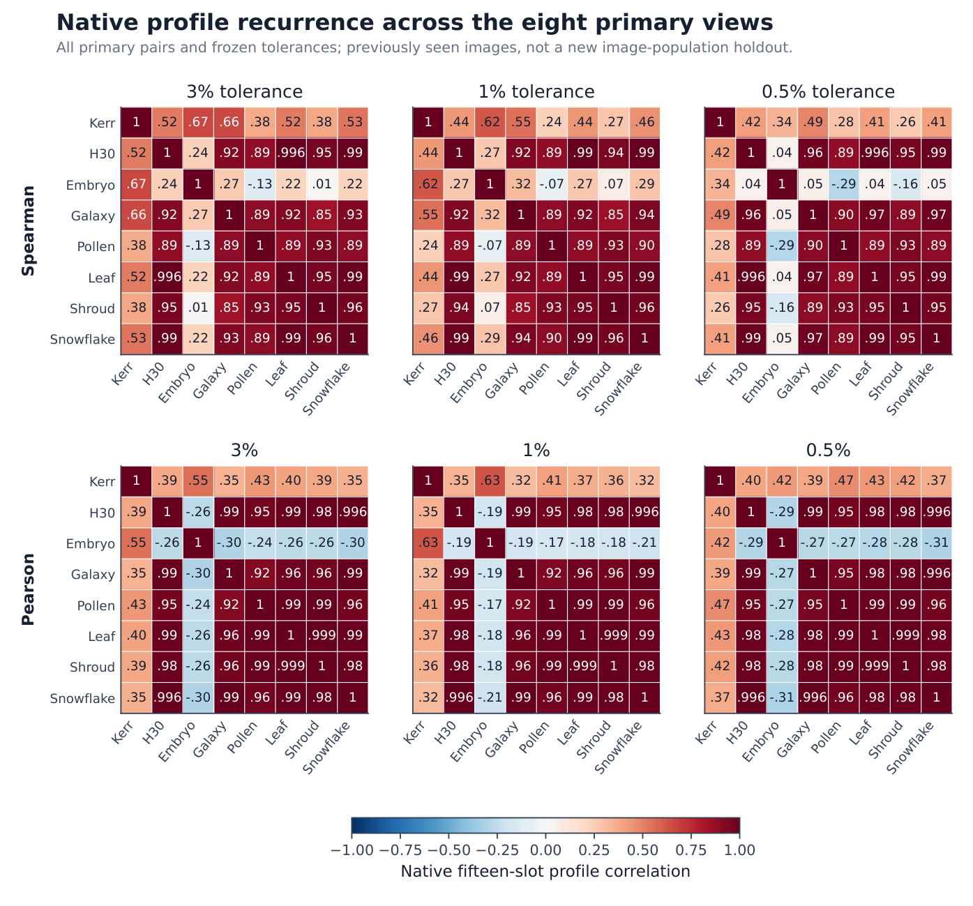
The observed comparison contains 17 views: Kerr, two hydrogen readouts and 14 spatial variants. The eight-view primary descriptive core contains Kerr, hydrogen log1p and six dark families. All identities, fifteen slots and three tolerances remain in the comparison. Figure 1 and [Appendix D](/source-readout/spectral-ratios/09-verification-and-appendices#appendix-d) show every core pair, including image–image comparisons. The public supplement includes all 17 views.

<a id="table-2"></a>

**Table 2. Primary hydrogen log1p versus six dark image signatures.** $F_{G,s}$ counts the fraction of all 10,000 paired-library coefficients at least the target, including target and ties.

| Source | Spearman 3% | Spearman 1% | Spearman 0.5% | Pearson 3% | 3% Spearman reference fraction |
| --- | ---: | ---: | ---: | ---: | ---: |
| Embryo | 0.23900 | 0.26856 | 0.04482 | -0.25984 | 0.54060 |
| Galaxy | 0.92063 | 0.92328 | 0.96373 | 0.98928 | 0.97900 |
| Pollen-like | 0.88641 | 0.88641 | 0.88518 | 0.95464 | 0.86000 |
| Leaf | 0.99553 | 0.99463 | 0.99642 | 0.98673 | 0.16900 |
| Shroud | 0.94868 | 0.94492 | 0.94765 | 0.97981 | 0.71350 |
| Snowflake | 0.98743 | 0.98652 | 0.98921 | 0.99637 | 0.44180 |

At 3%, five hydrogen–image Spearman coefficients span 0.886 to 0.996. They remain between 0.885 and 0.996 at narrower widths. Embryo dark is the clear exception, at 0.239, 0.269 and 0.045, with negative Pearson coefficients at all widths. Its bright version differs strongly but remains a sensitivity view. Pairwise agreement among the five other primary images is also high: the 3% Spearman range is 0.851–0.988. The recurrence is broad and heterogeneous.

Kerr is more moderately related. Its 3% Spearman coefficients are 0.52143 with hydrogen, 0.66848 with embryo, 0.65708 with galaxy, 0.38277 with pollen-like microscopy, 0.52189 with leaf, 0.38399 with Shroud and 0.53335 with snowflake. The full comparisons retain each of these pairs and their narrower-width results.

<a id="figure-1"></a>

<figure>
<img src="/publications/spectral/spectral-ratios/figure-1.png" alt="Six heat maps compare all eight primary views at three tolerances. Five image families agree strongly with hydrogen; dark embryo is the exception and Kerr agreement is more moderate." />
<figcaption>Figure 1. Complete primary-core profile comparisons at all three tolerances. Spearman is primary descriptive and Pearson secondary. The fifteen incidence slots retain ties and algebraic dependence. These are value-ratio profile correlations, not adjacent-gap statistics, null-excess correlations or repeats of earlier full-histogram correlations. The exact coefficients are in Table 6.</figcaption>
</figure>

<a id="section-5-2"></a>

### Similar profiles also occur under alternative libraries

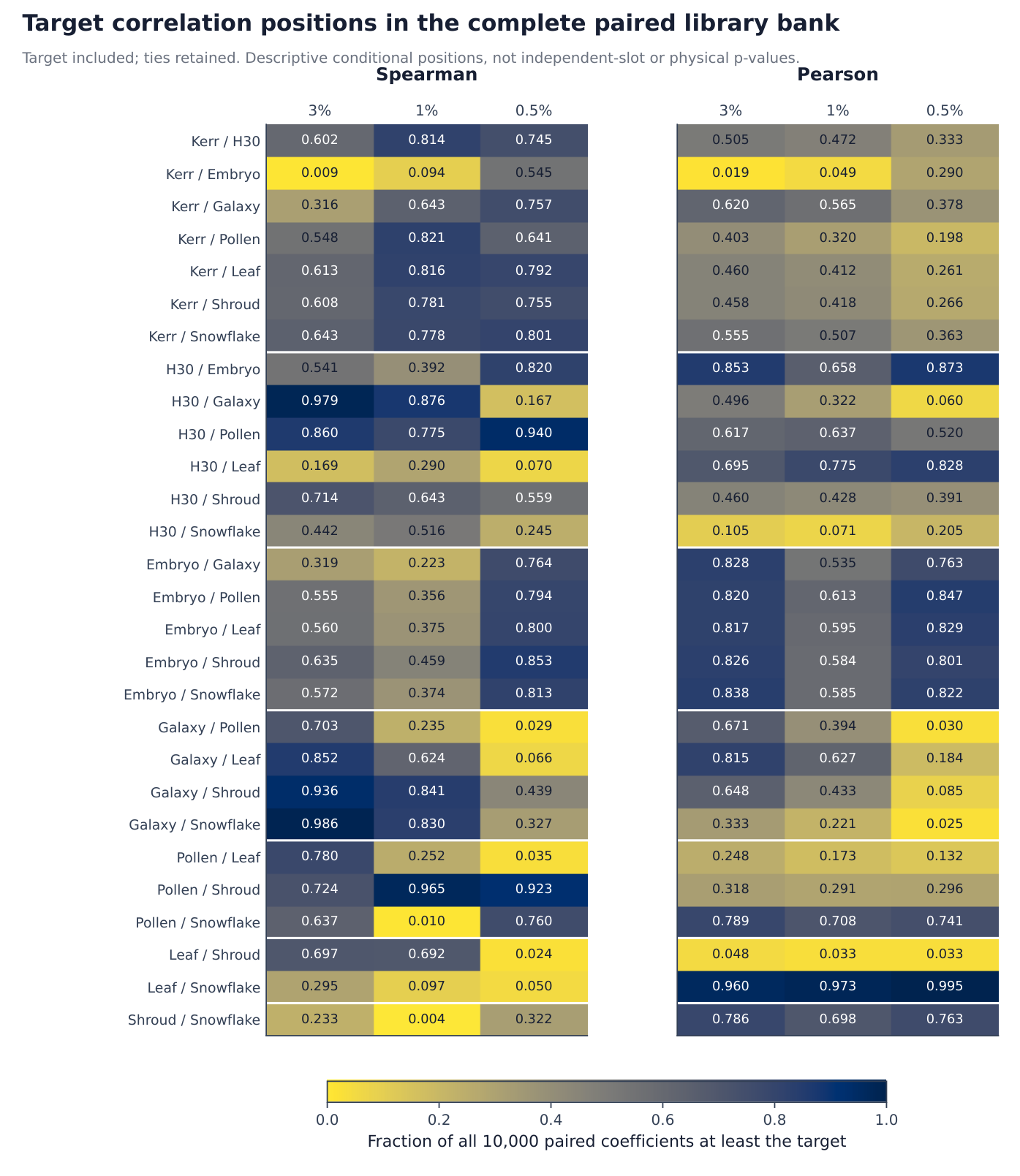
For hydrogen versus the six dark families, the 36 coefficient/tolerance comparisons give conservative fractions at least the target from 0.0598 to 0.9790. Strong recurrence in native profiles does not establish that the target library has an exceptional correlation in this bank.

Kerr–embryo at 3% is an exception to that general pattern. Its Spearman coefficient is 0.66848 with reference fraction 0.0086; Pearson is 0.54929 with fraction 0.0190. The distinction weakens at narrower widths. This is descriptive among the many retained pairs, not a replacement primary test. Both conservative fractions and symmetric midpositions are supplied because exact ties can be substantial. No new selected significance threshold is imposed.

<a id="figure-2"></a>

<figure>
<img src="/publications/spectral/spectral-ratios/figure-2.png" alt="Color-coded matrix of the fractions of paired library correlations that equal or exceed the target for each core pair and window width." />
<figcaption>Figure 2. Every primary-core target coefficient's position in the complete paired alternative-library population. Fractions include the target and ties. They describe retained-bank specificity, not physical discovery probabilities or independent image replications. All 28 pairs, three widths and both coefficients are shown; Table 6 gives the exact values.</figcaption>
</figure>



## Where conditional discrimination survives

<a id="section-6"></a>

## Conditional discrimination and profile robustness

<a id="section-6-1"></a>

### Kerr's successes and the holdout boundary

At the frozen 3% SUM point,

<a id="kerr-incidences"></a>

$$
A_3^{\mathrm{dev}}=\frac{83{,}194}{272{,}049}=0.3058052,\qquad
A_3^{\mathrm{hold}}=\frac{138{,}984}{436{,}928}=0.3180936.
$$

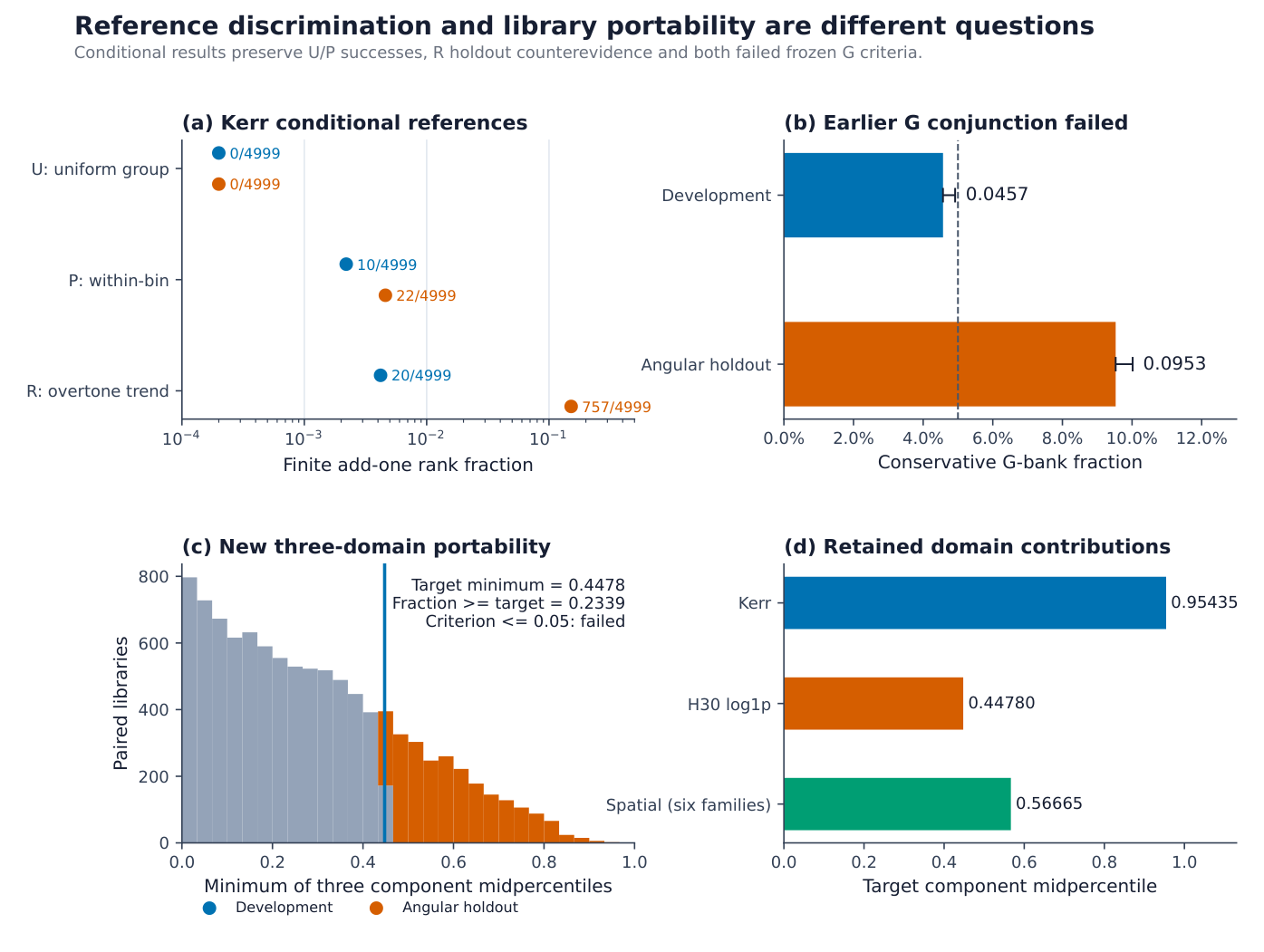
None of the 4,999 U controls reaches either observation. Under P, only 10 in development and 22 in holdout reach it. Both references discriminate the observed incidence strongly. P's distinction is especially informative because it preserves every labeled coarse raw-log bin and within-block circular difference.

<a id="table-3"></a>

**Table 3. Kerr conditional comparisons.** Each row has $B=4{,}999$. $\Delta A$ is observed incidence minus reference mean. Add-one fractions are conditional-reference summaries, not probabilities that a physical hypothesis is false.

| Data | Reference | Exceedances | Add-one fraction | Mean incidence | Difference |
| --- | --- | ---: | ---: | ---: | ---: |
| Development | U | 0 | 0.0002 | 0.24540 | 0.06041 |
| Holdout | U | 0 | 0.0002 | 0.24468 | 0.07341 |
| Development | P | 10 | 0.0022 | 0.26680 | 0.03901 |
| Holdout | P | 22 | 0.0046 | 0.26506 | 0.05304 |
| Development | R | 20 | 0.0042 | 0.28062 | 0.02518 |
| Holdout | R | 757 | 0.1516 | 0.31049 | 0.00760 |

The R holdout result is consequential: 757 controls reach the observation versus 20 in development. The experiment does not demonstrate strong holdout discrimination beyond the retained overtone trends and Gram structure. The nonnested laws do not identify a unique causal layer or eliminate every noise or artifact explanation across domains.

<a id="section-6-2"></a>

### Hydrogen shape withstands shell-block permutation

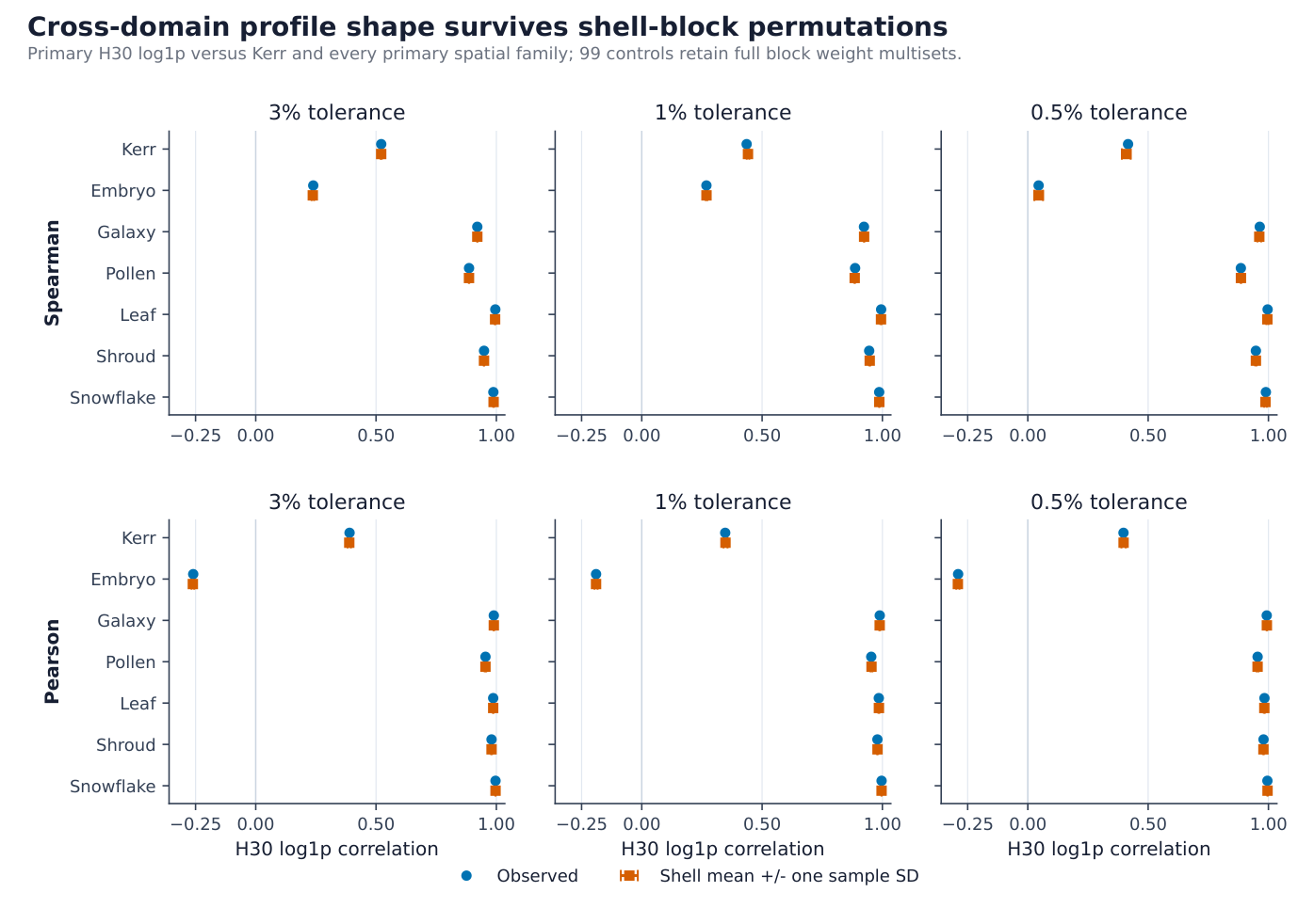
Relative shell-permutation displacement of the edge-weight vector is substantial, approximately $0.562$–$0.648$. Yet the hydrogen–Kerr Spearman coefficient is 0.521429 at the observation versus a shell mean of 0.521370, SD 0.002551. The difference is just 0.02297 sample SD. The six primary image coefficients are similarly close to their shell means.

<a id="table-4"></a>

**Table 4. Primary hydrogen log1p at 3%.** Native cross-domain Spearman coefficients and 99 shell-permutation replacements, with the other views held observed. Sample SD describes endpoint variability, not confidence intervals for independent sources.

| Other view | Observed | Shell mean | Sample SD | Standardized difference |
| --- | ---: | ---: | ---: | ---: |
| Kerr | 0.52143 | 0.52137 | 0.00255 | 0.02297 |
| Embryo | 0.23900 | 0.23732 | 0.00506 | 0.33137 |
| Galaxy | 0.92063 | 0.92081 | 0.00040 | -0.45749 |
| Pollen-like | 0.88641 | 0.88634 | 0.00094 | 0.07218 |
| Leaf | 0.99553 | 0.99479 | 0.00196 | 0.37787 |
| Shroud | 0.94868 | 0.94864 | 0.00090 | 0.04428 |
| Snowflake | 0.98743 | 0.98848 | 0.00169 | -0.62409 |

<a id="figure-3"></a>

<figure>
<img src="/publications/spectral/spectral-ratios/figure-3.png" alt="Shell means and sample standard deviations remain close to observed hydrogen correlations across seven comparisons, three tolerances and both coefficient types." />
<figcaption>Figure 3. Observed primary hydrogen–Kerr and hydrogen–six-dark-image coefficients against the means and sample SDs of all 99 shell replacements at each width. Both Spearman and Pearson are shown. The other view is held observed. Persistence is conditional on retained block multisets. The raw secondary and sensitivity-view comparisons are in the public supplement.</figcaption>
</figure>

Detailed shell-block structure remains in this perturbation. The result establishes neither random-matrix spectral rigidity nor the removal of all quantum and radial structure. At 3%, the cross-domain differences span $-0.624$ to $+0.378$ sample SD for Spearman and $-0.347$ to $+0.254$ for Pearson. The raw/log, width, coefficient and sensitivity comparisons are retained in the supplement; raw results do not follow by inference from the transformed view.

Each replacement changes just one hydrogen view while holding Kerr, the images and the other hydrogen view observed. That is not joint uncertainty across domains. Native $h/N_R$ correlation is different from correlation of $p-\mathbb E_0p$ or of standardized null excess. The paired per-library and per-slot Kerr and spatial null moments are absent here. Hydrogen null moments cannot substitute for them, and their absence does not erase the separate Kerr reference results.

<a id="section-6-3"></a>

### Hydrogen abundance changes with the readout

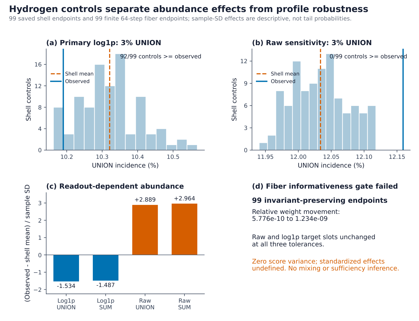
Raw 3% UNION is $26{,}122/214{,}832=0.1215927$. Its shell mean is $0.1203374$, SD $0.00043448$. No retained endpoint reaches the observation, giving descriptive $\Delta/s=+2.88916$. Primary transformed UNION is $21{,}892/214{,}832=0.1019029$, below its shell mean of $0.1032113$, SD $0.00085315$. Its $\Delta/s=-1.53358$, and 92 of 99 endpoints reach it. SUM shows the same readout-dependent signs. Raw abundance discrimination and transformed profile robustness answer different questions.

<a id="table-5"></a>

**Table 5. Hydrogen shell controls at 3%.** Every row uses 214,832 ordered nonself pairs. The standardized differences describe finite pilots, not calibrated extreme tails.

| Readout | Count | Observed | Shell mean | Sample SD | Standardized difference | Reaches observation |
| --- | --- | ---: | ---: | ---: | ---: | ---: |
| log1p | UNION | 0.101903 | 0.103211 | 0.000853 | -1.53358 | 92/99 |
| Raw | UNION | 0.121593 | 0.120337 | 0.000434 | 2.88916 | 0/99 |
| log1p | SUM | 0.109365 | 0.110799 | 0.000965 | -1.48664 | 91/99 |
| Raw | SUM | 0.129650 | 0.128180 | 0.000496 | 2.96446 | 0/99 |

The short fiber endpoints move only $5.78\times10^{-10}$ to $1.23\times10^{-9}$ relative to the parent. Although all 99 spectra are distinct at the numerical tolerance, all 90 target slot/readout/width incidences stay fixed. Both aggregate statistics and all 204 target conditional coefficient summaries have zero sample variance. The actual-statistic informativeness gate fails. The standardized effects are undefined. A short restarted run can preserve extra fine structure by locality; this pilot certifies neither mixing nor sufficiency of its named constraints.

<a id="figure-4"></a>

<figure>
<img src="/publications/spectral/spectral-ratios/figure-4.png" alt="Raw and log1p hydrogen incidence fall on opposite sides of their shell means. The short fiber control moves weights negligibly and has zero target score variance." />
<figcaption>Figure 4. Panels (a,b) show all 99 transformed and raw UNION outcomes separately. Panel (c) compares the corresponding UNION and SUM standardized differences. Panel (d) shows the fiber pilot's negligible motion and zero target score variance. No normal-tail extrapolation is made.</figcaption>
</figure>



## What the recurrence does and does not explain

<a id="section-7"></a>

## Library specificity fails its frozen test

The target midpositions are $P_K=0.95435$, $P_H=0.44780$ and $P_I=0.56665$. Their minimum is $Q=0.44780$. In the target-plus-$G$ population, 23.39% reach or exceed this minimum. That is above the frozen $F_Q\le0.05$ criterion. The original fifteen centers do not demonstrate an unusual simultaneous advantage across all three native domains.

The earlier Kerr-only test also misses its frozen conjunction. The $G$ ranks were 457/10,000 in development and 953/10,000 on angular holdout, with add-one fractions 0.0457 and 0.0953. One-sided 95% upper bounds were approximately 0.04919 and 0.10018. Both had to meet the 5% criterion. The target still exceeds the $G$ means by 0.03141 and 0.03323 incidence units respectively. Higher absolute incidence on holdout does not rescue the rank prediction. The secondary $S$ ranks, 135 and 743, also miss top-5% holdout performance.

The failed tests limit a library advantage. They do not negate the measured recurrence or the U/P discrimination. Conversely, those positive results do not establish a universal replacement. The alternative library was mechanically matched in Kerr, and its density-weighted effects on another operator remain empirical comparisons rather than a derived coordinate mapping.

<a id="figure-5"></a>

<figure>
<img src="/publications/spectral/spectral-ratios/figure-5.png" alt="The Kerr reference test succeeds against U and P but is weaker against R on holdout. The earlier two-dataset and later three-domain library criteria both fail." />
<figcaption>Figure 5. Panel (a) compares the U/P/R reference fractions. Panel (b) shows earlier G-bank add-one rank fractions and one-sided 95% Clopper–Pearson upper bounds against the 5% line. Panels (c,d) show the paired-G minimum and target component positions using development Kerr and six previously seen image families. Conditional discrimination and frozen library specificity are distinct tests.</figcaption>
</figure>

<a id="section-8"></a>

## Which spectral theories could explain this profile?

<a id="section-8-1"></a>

### Consecutive gaps are a complementary observable

For ordered levels $E_1<\cdots<E_n$, Atas et al. [\[1\]](/source-readout/spectral-ratios/09-verification-and-appendices#ref-1) use gaps $s_i=E_{i+1}-E_i$, consecutive ratios $r_i=s_i/s_{i-1}$, and folded ratios $\widetilde r_i=\min(r_i,r_i^{-1})$. A gap ratio uses three adjacent levels. With 464 distinct levels it yields 462 overlapping observations, instead of the 214,832 ordered value ratios here. Positive affine changes $E\mapsto aE+b$ leave the gap ratios unchanged. All-pair value ratios are scale-invariant and generally shift-sensitive.

A common local spacing scale cancels, allowing useful comparisons without explicit unfolding. Arbitrary nonlinear transforms are not exactly invisible: this cancellation is local when the density or transformation changes slowly across neighboring gaps. Symmetry sectors, unresolved degeneracies, spectral edges and finite-size effects require separate treatment. Atas et al. resolve translation sectors in the Ising example. The mere real symmetry of a structured graph does not establish GOE statistics.

The Gaussian-ensemble three-level surmise is

<a id="eq-15"></a>

$$
P_\beta(r)=\frac{(r+r^2)^\beta}{Z_\beta(1+r+r^2)^{1+3\beta/2}},\qquad \beta=1,2,4. \tag{15}
$$

A stationary Poisson level process gives $P(r)=(1+r)^{-2}$. The GOE folded-mean surmise $4-2\sqrt 3\simeq0.53590$ differs from the reported large-matrix numerical mean near 0.5307. The paper gives an exact limiting GUE comparison via the sine-kernel process and documents finite-size corrections. These are gap-ratio laws, not predictions for arbitrary all-pair value-ratio window masses. This investigation ran no gap-statistics experiment on the present spectra.

<a id="section-8-2"></a>

### Global density and local universality can vary independently

Levi and Oz [\[2\]](/source-readout/spectral-ratios/09-verification-and-appendices#ref-2) study feature-feature sample covariance $\Sigma_M=XX^\top/M$ with columns of $X\in\mathbb R^{d\times M}$ representing centered, normalized samples. Natural-image datasets show the bulk rank law $\lambda_i\propto i^{-1-\alpha}$, separate from leading outliers and small-eigenvalue tails. Their correlated Gaussian model takes a positive diagonal population covariance from the singular values of the Toeplitz construction $T_{ij}=I_{ij}+c|i-j|^\alpha$. Its sample covariance is Wishart. Generalized Marchenko–Pastur theory models density conditional on the population covariance and aspect ratio $d/M$.

Correlated and uncorrelated Gaussian samples can share GOE gap statistics while exhibiting different global densities. Appendix C of their paper shows that a deterministic population spectrum can reproduce broad scaling and miss local sample-covariance spacings. Appendix D finds scaling changes under augmentation while local gaps are comparatively stable. Appendix E separates eigenvector localization and alignment from density. Appendix F uses the model predictively for learning curves with bulk, sampling and basis assumptions.

The operators here are single-image distance-graph Laplacians, a radial coupling graph and a transformed damping spectrum. The graph identity $L=B\operatorname{diag}(w)B^\top$ is a Gram factorization, but incidence columns are constrained, sparse and dependent; weights encode declared structure; and $L\mathbf 1=0$. The factorization supplies neither independent Gaussian samples nor a Wishart asymptotic regime. A bulk covariance law also does not cover the entire retained positive spectrum or its nonlinear minimum-dependent readout automatically. Neither cited work validates a quantitative prediction for these profiles.

<a id="section-8-3"></a>

### A density explanation needs independent window predictions

An independently specified smooth log-native density $f$ under an additional iid distinct-value approximation gives

<a id="eq-16"></a>

$$
g(t)=\int f(u)f(u-t)\,du,\qquad q_j=\frac{\int_{I_j\cap B}g(t)\,dt}{\int_B g(t)\,dt}. \tag{16}
$$

For uncut positive values with density $p$ and CDF $F$, this is equivalently

<a id="eq-17"></a>

$$
q_j=\int_0^\infty p(y)\left\{F[c_j(1+\epsilon)y]-F[c_j(1-\epsilon)y]\right\}\,dy. \tag{17}
$$

For fixed unfiltered $n$, the iid expected hit count is $n(n-1)q_j$. With random filtered exposure, [Equation (16)](/source-readout/spectral-ratios/07-specificity-and-explanatory-tests#eq-16) gives a population conditional-pair probability or ratio of expected counts, not generally $\mathbb E[h_j/N_R]$.

Constrained finite ensembles can have the same mean one-point counting density $\rho_1$ and different factorial two-point intensity $\rho_2$. Exact expected nonself counts integrate $\rho_2$. Even fixed-$n$ iid values give $\rho_2(x,y)=(n-1)\rho_1(x)\rho_1(y)/n$. Dropping the factor corresponds to Poisson-number or asymptotic factorization. Connected correlations, variation between realization densities and extrema constraints can matter. In particular, hydrogen's [Equation (3)](/source-readout/spectral-ratios/02-native-operators#eq-3) fixes $v_{\min}=\ln 2$ and $u_{\min}=\ln\ln 2$; retain the anchor and its finite pair weights.

Global density is a candidate explanation once a model and quantitative window predictions are specified. Local gap correlations supply different information. Replaying the measured spectrum by the exact autocorrelation identity is not an independent prediction. Appendix C gives a closed-form illustration without claiming a fit or test on these spectra.



## A reproducible diagnostic and the next test

<a id="section-9"></a>

## What the experiment establishes

The positive contribution is a reproducible cross-operator comparison of finite structural signatures, with distinct results for recurrence, robustness and conditional discrimination. Primary transformed hydrogen and five image graphs give the strongest recurring shape. The embryo exception and moderate Kerr associations locate its heterogeneity. Kerr's U/P results exceed the specified uniform-group and coarse-bin/phase references. Shell-block stability demonstrates robustness to changes in weight placement that preserve detailed block multisets. The failed joint specificity criterion leaves those findings intact.

The signatures are functionals of spectral multisets. Isospectral operators necessarily give identical signatures. Fifteen windows cannot restore information already absent from the spectrum. Log autocorrelation also loses translation and phase information. A signature can register geometry carried through the spectrum without identifying a unique geometry or eigenbasis. The measured coefficients establish no common physical carrier, physical realization law, universal sign inversion between coherence and dissipation, or uniquely selected invariant. In particular, preserving a weight histogram need not destroy relevant physical structure: shell multisets retain detailed radial information.

The contribution can develop in three directions: cross-operator application, a compact density-sensitive descriptor alongside gap statistics, or reproducible residuals beyond a separately specified density-and-pair model. General classification and added value over density, quantile, moment or spacing summaries would require an explicit task and independent objects. A different observable by itself does not establish novelty. An ordinary density mechanism would not erase its possible diagnostic value. The two-paper comparison is not an exhaustive priority search.

A bounded next calculation would fit a fixed low-complexity density model using the saved hydrogen shell spectra and test it against the retained tables. Declare the endpoint split, propagate fit uncertainty, preserve the minimum anchor, and keep all fifteen slots and all three widths. The already seen endpoints make that an exploratory calibration. Separate adjacent-gap calculations could ask whether local correlations change while the all-pair profile survives; declare coordinate choice, sectors and degeneracy rules in advance. Neither extension was executed. For independent explanation, derive density from operator parameters or separate objects and validate on new objects. Broader universality and physical interpretation remain questions for those tests.

<a id="section-10"></a>

## The result in full scope

Finite recurrence is strong in several specified constructions, heterogeneous, and generally shared by alternatives. Kerr distinguishes two nominated references in development and holdout, with weaker holdout separation from the overtone/Gram-preserving law. Hydrogen profile shape survives shell-block permutation, but aggregate abundance depends on the readout and the short fiber pilot is uninformative. The frozen joint library test fails at 0.2339.

The log-autocorrelation representation identifies precisely what is being measured and what an explanatory density model must predict. It does not turn the comparison into a common physical mechanism. Related random-matrix results do not already explain these operators quantitatively. Independent prediction, independent-object testing and utility comparisons are the direct next steps.

<a id="data-code"></a>

## Data and code availability

The public verification supplement supplies retained inputs, library definitions, compact controls, result tables, executable verification and regeneration code, plot scripts, dependency pins and checksums. Its README separates quick checks on stored results from full numerical regeneration and reports actual executions. Billions of repeated derived matrix cells are reconstructed or recomputed in batches rather than stored. The original publication preparation did not run a clean full numerical reproduction or start a new scientific campaign.

Spatial numerical replay begins with the retained centroids. The supplement excludes photographs, thumbnails and overlays. It retains exact hashes, known acquisition identifiers and extraction rules. Six exact mappings and all seven photographic permission records are unresolved. Fully independent acquisition and pixel replay are therefore not represented as public or complete.

The supplied manuscript labels [10.5281/zenodo.23888292](https://doi.org/10.5281/zenodo.23888292) a reserved publication identifier and does not assert public upload at the time of preparation. The author's research platform is [everythingequation.com](https://www.everythingequation.com). The new author-created text, figures and tables are licensed CC BY 4.0; the adaptation retains the provenance and limits of the source.

<a id="author-statement"></a>

## Author statement

Jeremy Rodgers developed the research programme and core manuscript. AI tools supported additional numerical work, cross-checking, literature reconciliation and editorial revision. The author retains responsibility for the interpretation and final manuscript.



## Verification, invariances and the complete comparison data

<a id="appendix-a"></a>

## Appendix A. Numerical conventions and verification

The cross-domain execution used Python 3.12.14, NumPy 2.3.5, SciPy 1.17.0 and Pillow 12.2.0. The earlier 4,999-control Kerr execution used NumPy 2.5.4. Keeping the actual control values distinguishes exact input preservation from a generator rerun whose results can vary by platform. The supplement records versions for the executable subset and plotting workflow.

Floating arrays use double precision and source hashes preserve state, point and library order. Counting uses eligible sorted ordered ratios and inclusive matching endpoints, without histogram binning or ratio rounding. Independent direct Boolean counters check selected complete fifteen-slot cases. The prepared-window acceleration matched every field in four complete 10,000-library reference cases at all widths, including overlap and boundary fixtures.

For spatial eigenvalues the zero threshold is $\max(10^{-12},10^{-12}\max_i|\lambda_i|)$. Hydrogen uses $50\epsilon_{\rm mach}N\max_i|\lambda_i|$ on the full $N=465$ spectrum. Each construction requires exactly one eigenvalue within its threshold and no eigenvalue below the negative threshold. Retained positive modes preserve multiplicity. Independent checks covered eigenpair residuals, orthogonality, centroid identities and counts.

The source software suite passed 118 tests. Final integrity checks authenticated 413 score datasets, 41,300 batches and 185,850,000 slot counts. Stored observed and conditional representations account for 401 full or losslessly reconstructable matrix stores. These are execution-coverage counts, not independent sample sizes. The public quick check is narrower than a clean rerun: it checks stored tables, definitions, counts, pairings, selected independent numerical reconstructions and the manuscript claim index. Full-regeneration commands are given separately, and source image acquisition remains gated. Platform and BLAS differences can alter last-bit eigenvalues, so use declared tolerances rather than bitwise equality for regenerated eigenspectra.

<a id="appendix-b"></a>

## Appendix B. Invariances and nonidentifiability

For symmetric nonnegative weights,

<a id="eq-18"></a>

$$
x^\top Lx=\frac12\sum_{i,j}W_{ij}(x_i-x_j)^2\ge0. \tag{18}
$$

Every connected support has the constant vector as its one-dimensional kernel. Multiplying all weights by a common positive factor scales positive eigenvalues and leaves raw and minimum-normalized log1p ratios unchanged. When the numerical protocol uses an absolute zero threshold, assume the same positive-mode set is retained. This invariance explains cancellation of a uniform coupling scale without deriving the coupling constant.

The complete Fejér readout is injective on positive scalar eigenvalues:

<a id="eq-19"></a>

$$
f_T'(\lambda)=\frac{(T\lambda+1)e^{-T\lambda}-1}{T\lambda^2}<0. \tag{19}
$$

For known $T$, the complete unnormalized values determine the positive eigenvalues. The operator-valued readout determines the operator by inverse functional calculus under the same spectral hypotheses. Pooling ratios or windowing removes some of this information. Survival-readout ratios $e^{-T\lambda_i}/e^{-T\lambda_j}$ instead encode differences and lose a common additive shift. These conditional inversion statements do not establish physical transport between systems.

The ordered ratio multiset is invariant under common positive scaling and $v_i\mapsto a/v_i$ for $a>0$: inversion exchanges pair orientations. The whole-multiset ambiguity survives any fixed cutoff even though an asymmetric cutoff breaks reciprocal balance of the conditioned distribution. More general log-autocorrelation ambiguities and coarse windows obstruct unique inversion further. A label permutation alone preserves the spectrum and ratios and is no substantive control for the pooled observable.

<a id="appendix-c"></a>

## Appendix C. A closed-form density illustration

Let a hypothetical continuous rank model be $v(k)=Ak^{-p}$ with $p>0$ and $k$ uniform on $[k_{\min},k_{\max}]$. After translation, the log-density is a truncated exponential with $a=1/p$ and $L=p\log(k_{\max}/k_{\min})$. Integrating the product of densities gives

<a id="eq-20"></a>

$$
g(t)=
\begin{cases}
\dfrac{a\left(e^{-a|t|}-e^{-2aL}e^{a|t|}\right)}{2(1-e^{-aL})^2}, & |t|\le L,\\
0, & |t|>L.
\end{cases}\tag{20}
$$

For $t\ge0$ the integral is proportional to $e^{-at}\int_0^{L-t}e^{-2au}\,du$. Symmetry supplies the negative half. Holding $L$ fixed, the $a\to0$ limit is $(L-|t|)/L^2$ on the interval. With rank bounds fixed, $p$ and $L$ are not independent. Integrate over [Equation (9)](/source-readout/spectral-ratios/03-exact-ratio-statistics#eq-9), including the actual cutoff, to predict window masses once a model is independently supplied. This illustrates a bridge from a broad rank law such as that in Levi and Oz [\[2\]](/source-readout/spectral-ratios/09-verification-and-appendices#ref-2); it was not fitted or numerically tested here. Using the observed spectrum instead returns the identity in [Equation (8)](/source-readout/spectral-ratios/03-exact-ratio-statistics#eq-8).

<a id="appendix-d"></a>

## Appendix D. All primary-core comparisons and native summaries

The 28 unique core pairs are retained at each of three tolerances. Table 6 includes both coefficient types and conservative paired-bank fractions. The full 17-view table, symmetric entries, statuses, conditional profile summaries and sensitivity results are supplied electronically. Table 7 gives native target incidence and bank midposition for all observed views. Native spatial abundance uses 1% UNION even when the shape comparison uses 3%.

<a id="table-6"></a>

**Table 6. Complete primary-core pair comparisons.** Spearman is primary descriptive and Pearson secondary. Fractions count all target-plus-G coefficients at least the corresponding target, with ties retained.

| Left | Right | Tolerance | Spearman | Spearman fraction | Pearson | Pearson fraction |
| --- | --- | --- | --- | --- | --- | --- |
| Kerr | H30 log 1p | 3% | 0.52143 | 0.60200 | 0.38983 | 0.50530 |
| Kerr | Embryo | 3% | 0.66848 | 0.00860 | 0.54929 | 0.01900 |
| Kerr | Galaxy | 3% | 0.65708 | 0.31630 | 0.34932 | 0.62020 |
| Kerr | Pollen | 3% | 0.38277 | 0.54830 | 0.43262 | 0.40290 |
| Kerr | Leaf | 3% | 0.52189 | 0.61290 | 0.40281 | 0.45970 |
| Kerr | Shroud | 3% | 0.38399 | 0.60770 | 0.38992 | 0.45810 |
| Kerr | Snowflake | 3% | 0.53335 | 0.64320 | 0.35456 | 0.55530 |
| H30 log 1p | Embryo | 3% | 0.23900 | 0.54060 | -0.25984 | 0.85300 |
| H30 log 1p | Galaxy | 3% | 0.92063 | 0.97900 | 0.98928 | 0.49600 |
| H30 log 1p | Pollen | 3% | 0.88641 | 0.86000 | 0.95464 | 0.61710 |
| H30 log 1p | Leaf | 3% | 0.99553 | 0.16900 | 0.98673 | 0.69500 |
| H30 log 1p | Shroud | 3% | 0.94868 | 0.71350 | 0.97981 | 0.46000 |
| H30 log 1p | Snowflake | 3% | 0.98743 | 0.44180 | 0.99637 | 0.10530 |
| Embryo | Galaxy | 3% | 0.26522 | 0.31930 | -0.30299 | 0.82760 |
| Embryo | Pollen | 3% | -0.13177 | 0.55510 | -0.23573 | 0.82000 |
| Embryo | Leaf | 3% | 0.22123 | 0.56050 | -0.25919 | 0.81670 |
| Embryo | Shroud | 3% | 0.01326 | 0.63510 | -0.26397 | 0.82550 |
| Embryo | Snowflake | 3% | 0.22484 | 0.57220 | -0.30057 | 0.83800 |
| Galaxy | Pollen | 3% | 0.89402 | 0.70270 | 0.91855 | 0.67060 |
| Galaxy | Leaf | 3% | 0.92145 | 0.85170 | 0.96477 | 0.81530 |
| Galaxy | Shroud | 3% | 0.85055 | 0.93580 | 0.95719 | 0.64790 |
| Galaxy | Snowflake | 3% | 0.92896 | 0.98590 | 0.99235 | 0.33340 |
| Pollen | Leaf | 3% | 0.88720 | 0.77980 | 0.98754 | 0.24830 |
| Pollen | Shroud | 3% | 0.93435 | 0.72360 | 0.98982 | 0.31790 |
| Pollen | Snowflake | 3% | 0.89443 | 0.63730 | 0.95739 | 0.78900 |
| Leaf | Shroud | 3% | 0.94953 | 0.69710 | 0.99863 | 0.04760 |
| Leaf | Snowflake | 3% | 0.98831 | 0.29460 | 0.98911 | 0.95950 |
| Shroud | Snowflake | 3% | 0.95727 | 0.23330 | 0.98489 | 0.78600 |
| Kerr | H30 log 1p | 1% | 0.43571 | 0.81390 | 0.34661 | 0.47240 |
| Kerr | Embryo | 1% | 0.62299 | 0.09380 | 0.62517 | 0.04940 |
| Kerr | Galaxy | 1% | 0.54927 | 0.64320 | 0.31747 | 0.56500 |
| Kerr | Pollen | 1% | 0.24175 | 0.82110 | 0.41242 | 0.32030 |
| Kerr | Leaf | 1% | 0.43828 | 0.81640 | 0.37102 | 0.41220 |
| Kerr | Shroud | 1% | 0.27482 | 0.78150 | 0.35665 | 0.41810 |
| Kerr | Snowflake | 1% | 0.45796 | 0.77810 | 0.31555 | 0.50690 |
| H30 log 1p | Embryo | 1% | 0.26856 | 0.39160 | -0.18999 | 0.65770 |
| H30 log 1p | Galaxy | 1% | 0.92328 | 0.87620 | 0.98887 | 0.32180 |
| H30 log 1p | Pollen | 1% | 0.88641 | 0.77540 | 0.95350 | 0.63680 |
| H30 log 1p | Leaf | 1% | 0.99463 | 0.28980 | 0.98493 | 0.77460 |
| H30 log 1p | Shroud | 1% | 0.94492 | 0.64310 | 0.97916 | 0.42810 |
| H30 log 1p | Snowflake | 1% | 0.98652 | 0.51560 | 0.99645 | 0.07060 |
| Embryo | Galaxy | 1% | 0.31795 | 0.22260 | -0.19019 | 0.53490 |
| Embryo | Pollen | 1% | -0.07420 | 0.35640 | -0.17174 | 0.61250 |
| Embryo | Leaf | 1% | 0.26904 | 0.37480 | -0.18236 | 0.59490 |
| Embryo | Shroud | 1% | 0.06933 | 0.45930 | -0.18215 | 0.58350 |
| Embryo | Snowflake | 1% | 0.28890 | 0.37400 | -0.20790 | 0.58520 |
| Galaxy | Pollen | 1% | 0.89484 | 0.23500 | 0.92326 | 0.39380 |
| Galaxy | Leaf | 1% | 0.92493 | 0.62390 | 0.96373 | 0.62700 |
| Galaxy | Shroud | 1% | 0.85324 | 0.84130 | 0.95848 | 0.43300 |
| Galaxy | Snowflake | 1% | 0.94139 | 0.83010 | 0.99261 | 0.22110 |
| Pollen | Leaf | 1% | 0.88799 | 0.25230 | 0.98970 | 0.17290 |
| Pollen | Shroud | 1% | 0.93011 | 0.96500 | 0.99050 | 0.29080 |
| Pollen | Snowflake | 1% | 0.89648 | 0.00960 | 0.95751 | 0.70830 |
| Leaf | Shroud | 1% | 0.94661 | 0.69210 | 0.99860 | 0.03340 |
| Leaf | Snowflake | 1% | 0.98828 | 0.09740 | 0.98733 | 0.97290 |
| Shroud | Snowflake | 1% | 0.95974 | 0.00370 | 0.98448 | 0.69800 |
| Kerr | H30 log 1p | 0.5% | 0.41644 | 0.74510 | 0.39744 | 0.33290 |
| Kerr | Embryo | 0.5% | 0.34075 | 0.54540 | 0.42209 | 0.29020 |
| Kerr | Galaxy | 0.5% | 0.48599 | 0.75700 | 0.38599 | 0.37830 |
| Kerr | Pollen | 0.5% | 0.28204 | 0.64100 | 0.47416 | 0.19790 |
| Kerr | Leaf | 0.5% | 0.40645 | 0.79230 | 0.43228 | 0.26110 |
| Kerr | Shroud | 0.5% | 0.25976 | 0.75470 | 0.41679 | 0.26570 |
| Kerr | Snowflake | 0.5% | 0.41300 | 0.80120 | 0.36863 | 0.36280 |
| H30 log 1p | Embryo | 0.5% | 0.04482 | 0.81960 | -0.28975 | 0.87260 |
| H30 log 1p | Galaxy | 0.5% | 0.96373 | 0.16670 | 0.99273 | 0.05980 |
| H30 log 1p | Pollen | 0.5% | 0.88518 | 0.93970 | 0.95481 | 0.51960 |
| H30 log 1p | Leaf | 0.5% | 0.99642 | 0.07010 | 0.98330 | 0.82800 |
| H30 log 1p | Shroud | 0.5% | 0.94765 | 0.55880 | 0.97940 | 0.39140 |
| H30 log 1p | Snowflake | 0.5% | 0.98921 | 0.24550 | 0.99552 | 0.20500 |
| Embryo | Galaxy | 0.5% | 0.05359 | 0.76390 | -0.27392 | 0.76320 |
| Embryo | Pollen | 0.5% | -0.28557 | 0.79360 | -0.27104 | 0.84700 |
| Embryo | Leaf | 0.5% | 0.04490 | 0.79960 | -0.28458 | 0.82850 |
| Embryo | Shroud | 0.5% | -0.15599 | 0.85300 | -0.27543 | 0.80080 |
| Embryo | Snowflake | 0.5% | 0.04523 | 0.81330 | -0.30535 | 0.82210 |
| Galaxy | Pollen | 0.5% | 0.90145 | 0.02900 | 0.95245 | 0.02970 |
| Galaxy | Leaf | 0.5% | 0.96546 | 0.06620 | 0.97699 | 0.18390 |
| Galaxy | Shroud | 0.5% | 0.89408 | 0.43940 | 0.97801 | 0.08500 |
| Galaxy | Snowflake | 0.5% | 0.97247 | 0.32650 | 0.99579 | 0.02540 |
| Pollen | Leaf | 0.5% | 0.88879 | 0.03490 | 0.99074 | 0.13160 |
| Pollen | Shroud | 0.5% | 0.93435 | 0.92280 | 0.99040 | 0.29580 |
| Pollen | Snowflake | 0.5% | 0.89117 | 0.75990 | 0.95625 | 0.74100 |
| Leaf | Shroud | 0.5% | 0.95123 | 0.02430 | 0.99855 | 0.03290 |
| Leaf | Snowflake | 0.5% | 0.98918 | 0.04960 | 0.98396 | 0.99540 |
| Shroud | Snowflake | 0.5% | 0.95434 | 0.32170 | 0.98285 | 0.76280 |

<a id="table-7"></a>

**Table 7. Native target views.** Midpositions refer to the same target plus 9,999 alternatives. The raw hydrogen readout, bright variants and adult portrait remain secondary.

| View | Eligible pairs | Window | Count | Incidence | Midposition |
| --- | --- | --- | --- | --- | --- |
| Kerr | 272049 | 3% | SUM | 0.30581 | 0.95435 |
| H30 log 1p | 214832 | 3% | UNION | 0.10190 | 0.44780 |
| H30 raw | 214832 | 3% | UNION | 0.12159 | 0.07820 |
| embryo | 870 | 1% | UNION | 0.05517 | 0.43155 |
| embryo bright | 1190 | 1% | UNION | 0.05042 | 0.95330 |
| galaxy | 11990 | 1% | UNION | 0.04370 | 0.55115 |
| galaxy bright | 93330 | 1% | UNION | 0.02674 | 0.50220 |
| pollen | 997002 | 1% | UNION | 0.02529 | 0.35660 |
| pollen bright | 1282556 | 1% | UNION | 0.03149 | 0.51300 |
| adult human | 2652 | 1% | UNION | 0.01357 | 0.17185 |
| adult human bright | 4830 | 1% | UNION | 0.05404 | 0.58295 |
| leaf | 325470 | 1% | UNION | 0.04696 | 0.60690 |
| leaf bright | 145542 | 1% | UNION | 0.02020 | 0.35485 |
| shroud | 153272 | 1% | UNION | 0.03982 | 0.69565 |
| shroud bright | 81510 | 1% | UNION | 0.04368 | 0.83610 |
| snowflake | 493506 | 1% | UNION | 0.03931 | 0.64350 |
| snowflake bright | 396270 | 1% | UNION | 0.04596 | 0.52875 |

<a id="appendix-e"></a>

## Appendix E. Material reconstruction corrections

<a id="table-8"></a>

**Table 8. Reconstructed H30 counts.** Exposure is 214,832 eligible ordered nonself ratios. The values replace earlier totals that were not recovered.

| Readout | 3% SUM | 3% UNION | 1% SUM | 1% UNION | 0.5% SUM | 0.5% UNION |
| --- | ---: | ---: | ---: | ---: | ---: | ---: |
| Raw | 27,853 | 26,122 | 9,186 | 9,186 | 4,563 | 4,563 |
| log1p | 23,495 | 21,892 | 7,800 | 7,800 | 3,895 | 3,895 |

The 465-state graph retains 464 positive modes and hence $464\times463=214{,}832$ ordered nonself pairs. The earlier 28,941/31,204 totals and denominator 214,576 do not reproduce under the declared minimum-normalized relative-window construction. The earlier fifteen marginals add to 30,264, below the purported 31,204 UNION, contrary to [Equation (7)](/source-readout/spectral-ratios/03-exact-ratio-statistics#eq-7). These numbers do not survive as established results. Minimum versus median normalization and log-distance versus relative windows explain some archived differences, but do not identify the lost 31,204 run. A common eigenvalue scale cannot change raw or own-minimum-normalized ratios.

Null-stage choices also matter. Retained raw-uniform controls gave raw UNION standardized difference approximately $-13.286$. Drawing uniform raw values then applying the primary transform gave about $+0.456$, whereas uniform sampling in the transformed range gave about $-21.562$. They are distinct reference laws. The unsupported historical H30 $+7.7$ claim is not used; shell preservation answers a separate question.

H12 is a separate 78-state construction with no same-$n$ links. It uses absolute radial amplitudes and an $m=0$ angular factor rather than squared radial weights. Its 506 edges, 77 positive modes, filtered exposures and counts cannot substitute for H30. Deterministic H12 count checks remain valid for H12. Missing random streams and phase conventions prevent transfer of stochastic or synthetic-generator claims. The present reconstruction likewise does not represent unrecovered historical image feature maps, sphere/speckle inputs or separate direct-distance protocols. It implies neither a universal physical/nonphysical boundary nor a synthetic-impossibility claim.

The electromagnetic Kerr local Fejér row has archived effect 12.2713 and width 2.3290. The gravitational row has archived effect 11.3464 and width 2.5887. A retained 100-draw plug-in uniform-Fejér bank at the same gravitational point gives 10.6137. These are distinct realizations. The local-scan original streams are unavailable, so the archived values are not represented as newly reproduced tail calibrations. The grouped-endpoint U reference with 4,999 draws and the R/P comparisons provide the explicit current conditional results.

<a id="references"></a>

## References

<a id="ref-1"></a>

**[1]** Y. Y. Atas, E. Bogomolny, O. Giraud, and G. Roux. “Distribution of the ratio of consecutive level spacings in random matrix ensembles.” Physical Review Letters 110, 084101 (2013). [DOI](https://doi.org/10.1103/PhysRevLett.110.084101).
<a id="ref-2"></a>

**[2]** Noam Itzhak Levi and Yaron Oz. “The underlying universal statistical structure of natural datasets.” Proceedings of the 42nd International Conference on Machine Learning, Proceedings of Machine Learning Research 267, pp. 34020–34043 (2025). [Article](https://proceedings.mlr.press/v267/levi25c.html).
<a id="ref-3"></a>

**[3]** Emanuele Berti, Vitor Cardoso, and Andrei O. Starinets. “Quasinormal modes of black holes and black branes.” Classical and Quantum Gravity 26(16), 163001 (2009). [DOI](https://doi.org/10.1088/0264-9381/26/16/163001).
<a id="ref-4"></a>

**[4]** Leo C. Stein. “qnm: A Python package for calculating Kerr quasinormal modes, separation constants, and spherical-spheroidal mixing coefficients.” Journal of Open Source Software 4(42), 1683 (2019). [DOI](https://doi.org/10.21105/joss.01683).
<a id="ref-5"></a>

**[5]** Fan R. K. Chung. Spectral Graph Theory. CBMS Regional Conference Series in Mathematics, vol. 92. American Mathematical Society, Providence, RI (1997). [DOI](https://doi.org/10.1090/cbms/092).