# Slow Passage and Prepared Hysteresis in Adaptive Spectral Carriers
A slow sweep delays switching past the static fold by a preparation-dependent amount. The prepared cycle has a nonzero geometric loop limit, while physical maintenance work grows as the sweep slows.
Jeremy Rodgers · 2026-11-04
DOI: https://doi.org/10.5281/zenodo.23935694
## A Slow Sweep Passes the Stationary Fold
## 1. Where switching happens
A stationary fold fixes the input at which an equilibrium ends. It does not fix the input at which a driven carrier leaves. As the restoring rate vanishes, the complete amplitude and memory can remain near the vanished state. The delay depends on the source dynamics, the incoming preparation and the observed exit surface. A full return requires capture by the other stable state after each local exit.
This is the same reciprocal carrier and external rate port as in the [sharp bistability analysis](/source-readout/sharp-uniqueness). Only the prescribed scalar input varies. The drive fixes spatial mode, phase and sweep; the reciprocal memory evolves the carrier. The analysis starts with an eight-coordinate source and separates one mixed critical coordinate from seven stable directions. It retains parameter motion and controls the stable error of a passing trajectory rather than assuming an attracting centre equilibrium.
Tracking the stable branch from a fixed distance selects an Airy solution and an oriented delay $K_f\nu^{2/3}+o(\nu^{2/3})$ at sufficiently small fixed exit levels. The example's unfitted prefactors are approximately 6.21890 and 7.91547. Starting exactly at the fold selects a different Airy mixture, with pole constant 1.98635 instead of 2.33811. Stationary memory substitution preserves folds yet changes dynamical coefficients. The proof then uses strict loss at fixed input for the connecting orbit, finite-time continuity for capture, and complete stable tracking through reversal. The resulting branch limit is uniform on compact input intervals away from switching and holds in finite-$L^p$ norms. It does not identify an exact vertical trace, a monotone amplitude jump or a finite-rate attracting periodic orbit. The oriented geometric loop has a positive limiting magnitude while physical maintenance work grows as $1/\nu$.
Four uninterrupted numerical cycles and preparation, uniqueness and modal controls evaluate this construction. The numerical thresholds are not assigned an analytically certified chart radius. The standard centre and Airy tools follow Carr (1981, 2006) and NIST (2026). The source contribution is a finite powered mechanism and explicit observation contracts. It does not establish a common microscopic law across atomic, image and Kerr readouts.
## 2. Time-dependent source, energy and boundedness
### 2.1 Complete state and prescribed input
Let $z\in\mathbb C^3$, $m\in\mathbb R^2$ and set
$$
b_1=(1,-1,0)^T,\quad b_2=(0,1,-1)^T,\quad B_e=b_eb_e^T,\quad L=B_1+B_2,\quad
K(m)=\mu I+\sum_{e=1}^2e^{m_e}B_e.\tag{1}
$$
$$
F(z,m)=\tfrac12z^*K(m)z+\tfrac\kappa2|m|^2,\qquad
g_e=\kappa m_e+\tfrac12e^{m_e}|b_e^Tz|^2.\tag{2}
$$
The positive parameters $\mu,\kappa,\gamma,\alpha,\eta$ stay fixed. Define $c=\gamma+i\alpha$ and the normalized highest path mode
$$
v_3=(1,-2,1)^T/\sqrt6.\tag{3}
$$
$$
\dot z=-cK(m)z+a(t)v_3,\qquad \dot m=-\eta g(z,m).\tag{4}
$$
Here $a(t)$ is real in the fixed phase reference. Both efforts derive from $F$, so memory is a free reciprocal source coordinate; $K(m)\ge\mu I$ at any finite state. Norms and joint Hessians use fixed Euclidean coordinates in amplitude, energy and time scales $A_0,E_0,T_0$. Before normalization, amplitude has units $A$, energy $E$, time $T$, $K$ has $E/A^2$, $\kappa$ has $E$, and $m$ is dimensionless. Both $\gamma,\alpha$ have $A^2/(ET)$ and $\eta$ has $1/(ET)$. Input and ramp rate have $A/T$ and $A/T^2$. Baseline edge weights equal one.
For $0
$$
a_\nu(t)=
\begin{cases}
a_\ell+\nu t,&0\le t\le T_h,\\
a_h-\nu(t-T_h),&T_h\le t\le2T_h,
\end{cases}\qquad T_h=(a_h-a_\ell)/\nu.\tag{5}
$$
Only the slope changes at reversal. There are no holds. Principal preparation is the low stationary state at $a_\ell$; perturbed preparations are identified separately. The experiment uses
$$
(\mu,\kappa,\gamma,\alpha,\eta)=(0.1,1,0.6,1.2,0.8),\qquad(a_\ell,a_h)=(2.9,3.17).\tag{6}
$$
### 2.2 Physical balance and the varying tilt
The rate $f=a(t)v_3$ pairs with conjugate effort $Kz$ (van der Schaft and Jeltsema, 2014). The external actuator can supply or absorb power; no finite reservoir is included.
$$
P(t)=\operatorname{Re}[(Kz)^*f(t)],\qquad \dot F=-\gamma\lVert Kz\rVert^2-\eta|g|^2+P.\tag{7}
$$
Put $\ell(t)=f(t)/c$ and $V(x,a)=F(z,m)-\operatorname{Re}[\ell(t)^*z]$. With
$$
q=(\operatorname{Re}z,\operatorname{Im}z),\quad x=(q,m),\quad
J=\begin{pmatrix}0&-I\\ I&0\end{pmatrix},\quad G=\gamma I+\alpha J,\quad
D=\operatorname{diag}(G,\eta I_2),\tag{8}
$$
the source is $\dot x=-D\nabla_x V(x,a(t))$. Both explicit parameter and state derivatives contribute almost everywhere:
$$
\dot V=-\gamma\lVert Kz-\ell\rVert^2-\eta|g|^2-\operatorname{Re}[\dot\ell^*z].\tag{9}
$$
At reversal $x,F,V$ remain continuous; [(9)](#eq-9) holds on each adjacent segment. The last term precludes assuming constant-input monotonicity along a ramp. Physical work obeys
$$
W(t)=\int_0^tP\,ds,\qquad
Q(t)=\int_0^t(\gamma\lVert Kz\rVert^2+\eta|g|^2)\,ds,\qquad
F(t)-F(0)=W(t)-Q(t).\tag{10}
$$
The tilted potential is not the stored energy of source or actuator.
**[Proposition 2.1](#proposition-2-1) (Bounded-input continuation).** Bounded piecewise continuous $f$ gives global forward evolution. At fixed initial state and $\lVert f\rVert\le f_{\max}$ the state bounds do not depend on ramp speed.
**Proof.** For $r_z=\lVert z\rVert$, Hermiticity and positivity give
$$
\tfrac12\frac d{dt}\lVert z\rVert^2\le-\gamma\mu\lVert z\rVert^2+f_{\max}\lVert z\rVert,\qquad
r_z(t)\le r_z(0)e^{-\gamma\mu t}+\frac{f_{\max}}{\gamma\mu}(1-e^{-\gamma\mu t}).\tag{11}
$$
The scalar bound holds in the upper Dini sense at zero. Set $Z=\max(r_z(0),f_{\max}/(\gamma\mu))$ and $M_e=\max(0,m_e(0))$. At zero memory its derivative is nonpositive; for positive memory $\dot m_e\le-\eta\kappa m_e$, so $m_e\le M_e$. Conversely,
$$
\dot m_e\ge-\eta\kappa m_e-\tfrac\eta2e^{M_e}\lVert b_e\rVert^2Z^2.\tag{12}
$$
$$
m_e(t)\ge m_e(0)e^{-\eta\kappa t}-\frac{e^{M_e}\lVert b_e\rVert^2Z^2}{2\kappa}(1-e^{-\eta\kappa t}).\tag{13}
$$
State smoothness and local Lipschitz continuity uniformly on compacts with bounded input, together with these bounds, exclude finite escape. Piecewise classical or absolutely continuous Carathéodory solutions continue through reversals. $\square$
At fixed drive [(9)](#eq-9) has strict loss except at equilibria. A nonstationary omega-limit point would imply a neighborhood of uniformly positive loss and infinitely many visits of uniformly positive duration, by bounded velocity, contradicting convergence of the tilt. The omega-limit set is connected by nested compact connected closures of forward tails. If stationary points are finite, each trajectory converges to one. This fixed-input invariance argument (LaSalle, 1976) will be used for a reference connection, not for ramp monotonicity.
## Complete Folds and the Mixed Critical Coordinate
## 3. Stationary geometry and complete fold data
At fixed amplitude the memory Hessian and stationary solution are
$$
(H_m)_{ee}=\kappa+\tfrac12e^{m_e}|b_e^Tz|^2>0.\tag{14}
$$
$$
m_e=-s_e,\quad s_ee^{s_e}=|b_e^Tz|^2/(2\kappa),\quad s_e=W_0(|b_e^Tz|^2/(2\kappa)).\tag{15}
$$
$$
V_{\rm eff}(z,a)=\tfrac\mu2\lVert z\rVert^2+
\sum_e\kappa(s_e+s_e^2/2)-\operatorname{Re}[(av_3/c)^*z].\tag{16}
$$
$W_0$ is the principal real Lambert function (Corless et al., 1996). This is an exact stationary correspondence. For $w=e^{-s}$ an edge has tangential curvature $w$ and radial curvature $-Q_0(s)$:
$$
Q_0(s)=e^{-s}\frac{s-1}{s+1},\quad Q_0'(s)=e^{-s}\frac{3-s^2}{(1+s)^2},\quad
\chi=(2-\sqrt3)e^{-\sqrt3}=\max_{s\ge0}Q_0(s).\tag{17}
$$
The orthonormal modes are $v_0=(1,1,1)^T/\sqrt3$, $v_1=(1,0,-1)^T/\sqrt2$ and $v_3$, with eigenvalues $0,1,3$.
**[Lemma 3.1](#lemma-3-1) (Complete counted regime).** For $\chi<\mu<3\chi$ and $a>0$, every stationary state has
$$
z=\theta R(s)v_3,\qquad m=(-s,-s),\qquad \theta=|c|/c,\quad R(s)=\sqrt{\tfrac{4\kappa}{3}se^s}.\tag{18}
$$
$$
a(s)=|c|\sqrt{H_3(s)},\qquad H_3(s)=\tfrac{4\kappa}{3}se^s(\mu+3e^{-s})^2.\tag{19}
$$
The two roots $s_-\in(1,\sqrt3)$ and $s_+>\sqrt3$ of $Q_0(s_\pm)=\mu/3$ give
$$
a_{\rm up}=a(s_-),\qquad a_{\rm down}=a(s_+),\qquad a_{\rm down}0$ since $Lv_1=v_1$. Its sole critical point is $h=0$. Both memory values then coincide; the amplitude equation fixes phase and gives [(18)](#eq-18)–[(19)](#eq-19). This excludes hidden complex or symmetry-broken equilibria. The derivative is
$$
H_3'(s)=\tfrac{4\kappa}{3}(\mu+3e^{-s})e^s(1+s)[\mu-3Q_0(s)].\tag{21}
$$
The unique maximum of $Q_0$ gives two simple turning points, maximum at $s_-$ and minimum at $s_+$. With $H_3(0)=0$ and $H_3(s)\to\infty$ the monotonic pieces give all counts. The complete Hessian is
$$
H=\begin{pmatrix}K_R&B\\ B^T&H_m\end{pmatrix},\qquad
K_R=\operatorname{diag}(K,K),\qquad B_{:e}=e^{m_e}\operatorname{diag}(B_e,B_e)q.\tag{22}
$$
Completing the memory square gives the negative and zero counts of $S=K_R-BH_m^{-1}B^T=\nabla^2V_{\rm eff}$ and two additional positive directions. At an equal-edge state the six Schur eigenvalues are
$$
\mu,\quad\mu-Q_0,\quad\mu-3Q_0;\qquad\mu,\quad\mu+w,\quad\mu+3w.\tag{23}
$$
The full mobility bridge applies because $H$ is symmetric and $\operatorname{Sym}D>0$. A nonzero imaginary eigenvector would give $(Hv)^*D(Hv)=-i\omega v^*Hv$, impossible by real parts. A generalized zero vector yields $0=-v_0^*D^{-1}v_0$ for $Hv_0=0$, impossible because $D^{-1}$ has positive symmetric part. Deforming $D$ to $I$ therefore preserves half-plane counts and zero multiplicity, including complex algebraic multiplicities. Equation [(23)](#eq-23) gives all stability classes. At a fold only $\mu-3Q_0$ vanishes, leaving seven decaying modes. The nonzero saddle-node coefficients follow next. $\square$
At either fold,
$$
X(x,a)=-DY(x,a),\quad Y(x,a)=\nabla F(x)-ah,\quad
h=(\operatorname{Re}(v_3/c),\operatorname{Im}(v_3/c),0,0).\tag{24}
$$
Let $x_f=x(s_f)$, $a_f=a(s_f)$ and $L_f=X_x(x_f,a_f)=-DH$. Normalize by
$$
r=x_s(s_f),\qquad d_f=r^TD^{-1}r>0,\qquad l^T=r^TD^{-1}/d_f,\qquad l^Tr=1.\tag{25}
$$
The two memory components of $r$ are $(-1,-1)$; neither amplitude quadrature nor memory is dropped. Differentiating the stationary identity at $a'=0$ gives $Hr=0$ and $r^TY_{xx}[r,r]=(r^Th)a''$; $r^Th=R'/|c|>0$. The full coefficients are
$$
A_f=l^TX_a=\frac{r^Th}{d_f}>0,\qquad B_f=\tfrac12l^TX_{xx}[r,r]=-\tfrac12A_f a''(s_f).\tag{26}
$$
From [(21)](#eq-21) $a''<0$ at $s_-$ and $a''>0$ at $s_+$. Thus $B_f$ is positive at the upper fold and negative at the lower fold. The simple zero and nonzero coefficients establish full saddle-nodes.
| Fold | $a_f$ | $A_f$ | $B_f$ | $K_f$ |
| --- | ---: | ---: | ---: | ---: |
| up | 3.105013621 | 0.398391766 | 0.133395769 | 6.218901175 |
| down | 2.958896746 | 0.355600158 | -0.072477106 | 7.915472816 |
**[Table 1](#table-1).** Complete fold coefficients for [(6)](/source-readout/slow-passage/01-source-and-energy#eq-6) with normalization [(25)](#eq-25). $K_f=\zeta_1/(A_f|B_f|)^{1/3}$. The computed stable gap is 0.06.
## 4. Fixed-fold reduction with dynamic memory
### 4.1 Projection and extended nilpotent structure
Fix $P_f=rl^T$, $Q_f=I-P_f$. Since $L_fr=0$ and $l^TL_f=0$, $E_s=\ker l^T$ is invariant and its restricted $A_s$ is Hurwitz. All coordinates are fixed at the fold:
$$
x-x_f=ry+w,\quad y=l^T(x-x_f),\quad w\in E_s,\quad \lambda=a-a_f.\tag{27}
$$
Input is affine and state independent, so $X_{xa}=0$. Taylor expansion gives
$$
\begin{aligned}
\dot y&=A_f\lambda+B_fy^2+N_y(y,w),\quad \dot w=A_sw+Q_fX_a\lambda+N_w(y,w),\\
N_y&=O(|y|^3+|y|\lVert w\rVert+\lVert w\rVert^2),\\
N_w&=O(y^2+|y|\lVert w\rVert+\lVert w\rVert^2).
\end{aligned}\tag{28}
$$
$$
\dot\lambda=\epsilon,\qquad \dot\epsilon=0.\tag{29}
$$
The augmented constant-slope system has centre coordinates $(y,\lambda,\epsilon)$ with a nilpotent linear chain $\dot y=A_f\lambda$, $\dot\lambda=\epsilon$, rather than three independent semisimple zero modes. The finite-dimensional centre-manifold theorem applies to the zero-real-part centre spectrum and strictly stable complement (Carr, 1981, 2006). Choose a finite $C^4$ chart and graph
$$
w=\psi(y,\lambda,\epsilon),\qquad \psi=O(y^2+|\lambda|+|\epsilon|).\tag{30}
$$
Inserting $\psi=C_\lambda\lambda+C_\epsilon\epsilon+\cdots$ in the invariance equation gives
$$
C_\lambda=\psi_\lambda(0)=-A_s^{-1}Q_fX_a,\qquad
C_\epsilon=\psi_\epsilon(0)=A_s^{-1}C_\lambda.\tag{31}
$$
The inverses act on $E_s$; $C_\epsilon$ retains parameter motion. The mixed critical equation becomes
$$
\dot y=A_f\lambda+B_fy^2+R,\qquad |R|\le C(|y|^3+|y\lambda|+\lambda^2+|\epsilon|).\tag{32}
$$
The graph retains dynamical memory rather than replacing it by a stationary Lambert value.
### 4.2 Attraction during passage
**[Lemma 4.1](#lemma-4-1) (Finite-chart stable-direction estimate).** In a sufficiently small fold chart the deviation $e=w-\psi(y,\lambda,\epsilon)$ decays exponentially for the time the complete trajectory stays in the chart, regardless of critical equilibrium stability.
**Proof.** Subtract the graph invariance equation at the actual $(y,\lambda,\epsilon)$. Parameter derivatives and the $B_fy^2$ term cancel:
$$
\dot e=A_se+[N_w(y,\psi+e)-N_w(y,\psi)]-\psi_y[N_y(y,\psi+e)-N_y(y,\psi)].\tag{33}
$$
The nonlinear derivatives in $w$ vanish at the origin and are $O(\delta)$ on a radius-$\delta$ chart; $\psi_y(0)=0$. Thus $\dot e=[A_s+O(\delta)]e+O(\lVert e\rVert^2)$. Choose $P_s>0$ on $E_s$ with $A_s^TP_s+P_sA_s=-I$. For small enough chart,
$$
\frac d{dt}(e^TP_se)\le-\tfrac12\lVert e\rVert^2.\tag{34}
$$
Norm equivalence gives $\lVert e(t)\rVert\le Ce^{-g(t-t_0)}\lVert e(t_0)\rVert$. Its effect on the critical equation is an integrable decaying perturbation. $\square$
After transients, variation of constants gives $w=O(\nu^{2/3})$ for $y=O(\nu^{1/3})$ and $\lambda=O(\nu^{2/3})$. If using moving stationary coordinates the forcing would include $-x_*'(a)\dot a$, and moving eigenvectors would add a connection term. The fixed chart avoids the singular branch derivative while keeping parameter motion in [(31)](#eq-31). Regular branch tracking below restores the moving-reference term explicitly.
## Preparation Selects the Airy Delay
## 5. Inner scaling and preparation-dependent passage
### 5.1 Orient the Riccati equation
Let $\sigma_f=\operatorname{sign}B_f$ and $b_f=|B_f|$.
$$
u=\sigma_f y,\qquad h=\sigma_f(a-a_f).\tag{35}
$$
On the outgoing leg $\dot a=\sigma_f\nu$, $\nu>0$, so $\dot h=\nu$ and
$$
\dot u=A_fh+b_fu^2+O(u^3+|uh|+h^2+\nu).\tag{36}
$$
Upper-fold delay means $a>a_{\rm up}$; lower-fold delay means $a
$$
t_\nu=(A_fb_f\nu)^{-1/3},\qquad
h_\nu=\frac{\nu^{2/3}}{(A_fb_f)^{1/3}},\qquad
u_\nu=\left(\frac{A_f\nu}{b_f^2}\right)^{1/3}.\tag{37}
$$
With $T=(t-t_f)/t_\nu=h/h_\nu$ and $U=u/u_\nu$, the inner equation on bounded $(T,U)$ sets after stable transients is
$$
\frac{dU}{dT}=T+U^2+O(\nu^{1/3}).\tag{38}
$$
The identities $\nu t_\nu=h_\nu$, $b_fu_\nu h_\nu=\nu$ fix the normalization. With dimensionless $u$, restored units of $A_f,b_f$ are $1/A,1/T$, and $t_\nu,h_\nu,u_\nu$ have units time, amplitude-rate and one. Positive rescaling of $r$ changes $A_f,b_f,u$ consistently and leaves $A_fb_f$ invariant. The fixed normalization is used in the projection measurements.
### 5.2 The incoming stable branch selects the solution
For $h<0$ the attracting stationary branch and restoring rate satisfy
$$
u_*(h)=-\sqrt{-A_fh/b_f}+O(h),\qquad
\lambda_c(h)=-2\sqrt{A_fb_f(-h)}+O(h).\tag{39}
$$
Preparation on this branch at fixed input distance gives regular tracking until a shrinking fold neighborhood. After fast errors settle, the critical error obeys
$$
D^+|e_c|\le-c_0\sqrt{-h}|e_c|+C\frac\nu{\sqrt{-h}}+C|e_c|^2.\tag{40}
$$
The moving reference has derivative $O((-h)^{-1/2})$; the stable block has a uniform gap and is controlled by [Lemma 4.1](/source-readout/slow-passage/02-folds-and-critical-coordinate#lemma-4-1). A sufficiently large $C_0$ makes $|e_c|\le C_0\nu/|h|$ invariant after the initial transient while $\nu/|h|^{3/2}$ is small. On its boundary restoring loss dominates forcing and quadratic error; boundary speed $O(\nu^2/|h|^2)$ is lower order. At overlap $h=-\nu^p$, $0
$$
U_\infty(T)=\frac{\operatorname{Ai}'(-T)}{\operatorname{Ai}(-T)},\qquad
U_\infty(T)\sim-\sqrt{-T}\quad(T\to-\infty).\tag{41}
$$
Indeed $U=-q'/q$ turns $U'=T+U^2$ into $q''+Tq=0$; $q(T)=\operatorname{Ai}(-T)$ has the incoming asymptotics, with the sign in [(41)](#eq-41) from differentiating $-T$. At fixed large entrance $T=-M$, [(40)](#eq-40) gives $U=-\sqrt M+O(M^{-1})+o(1)$ as $\nu\to0$. Along the negative branch sensitivity contracts by $\exp(\int 2U\,dT)$, of order $\exp(-4M^{3/2}/3)$ to a fixed inner interval. First let $\nu\to0$ on compact intervals, then $M\to\infty$. This selects [(41)](#eq-41), unlike setting $U(0)=0$.
**[Theorem 5.1](#theorem-5-1) (Tracked-preparation local delay).** At either complete fold, prepare on the incoming attracting branch at fixed positive input distance, or in a sufficiently small fixed attracting neighborhood there. Let $\dot a=\sigma_f\nu$ through the fold. For sufficiently small fixed outgoing level $d>0$, the first crossing at $a_d$ of
$$
u=\sigma_f l^T(x-x_f)=d\tag{42}
$$
after incoming and stable-direction transients satisfies
$$
\sigma_f(a_d-a_f)=K_f\nu^{2/3}+o(\nu^{2/3}),\quad
K_f=\frac{\zeta_1}{(A_fb_f)^{1/3}},\quad \zeta_1=2.338107410459\ldots,\tag{43}
$$
where $\operatorname{Ai}(-\zeta_1)=0$ is the first zero in positive $T$.
**Proof.** On compact intervals $T<\zeta_1$, matching and continuous dependence in [(38)](#eq-38) give $U\to U_\infty$, so $u=O(u_\nu)\to0$ cannot reach fixed positive $d$. For the upper bound choose large outgoing $M$ and $T_M<\zeta_1$ with $U_\infty(T_M)=M$. Inner convergence gives the crossing $u=Mu_\nu$ at $T\to T_M$. Bootstrap $h\le C_1h_\nu$ up to $d$. Choose $d$ small enough that the cubic term is bounded by $b_fu^2/4$. The remaining terms divided by $u^2$ are controlled by $h/u,h^2/u^2,\nu/u^2$, tending to zero at fixed $M$; $A_fh$ helps on this positive-$h$ interval. Therefore $\dot u\ge b_fu^2/2$, giving
$$
\Delta t\le\frac2{b_fMu_\nu},\qquad \frac{\Delta h}{h_\nu}\le\frac2M.\tag{44}
$$
This closes the bootstrap for fixed $C_1$. The limsup of the scaled exit is at most $T_M+2/M$. Sending $M\to\infty$ gives $\zeta_1$. This proves the smaller-order remainder, without an explicit full-source finite-rate constant. $\square$
### 5.3 Exact-fold and finite-inner preparations
For finite initial $(T_0,U_0)$ the quadratic solution is
$$
U(T)=\frac{\operatorname{Ai}'(-T)+k\operatorname{Bi}'(-T)}
{\operatorname{Ai}(-T)+k\operatorname{Bi}(-T)},\qquad
k=\frac{\operatorname{Ai}'(-T_0)-U_0\operatorname{Ai}(-T_0)}
{U_0\operatorname{Bi}(-T_0)-\operatorname{Bi}'(-T_0)}.\tag{45}
$$
If the ratio is not finite, use the proportional Airy combination directly. The first forward zero of its denominator determines passage when the preparation is in the outgoing class. Starting exactly at $x_f,a_f$ gives $T_0=U_0=0$, with distance $O(\nu)$ from the moving graph by [(31)](/source-readout/slow-passage/02-folds-and-critical-coordinate#eq-31), smaller than the inner critical scale. The Airy initial values give $k=1/\sqrt3$ and
$$
\operatorname{Ai}(-\zeta_0)+\operatorname{Bi}(-\zeta_0)/\sqrt3=0,\qquad
\zeta_0=1.986352707430\ldots.\tag{46}
$$
The same compact-inner and exit bounds give
$$
\sigma_f(a_d-a_f)=\frac{\zeta_0}{(A_fb_f)^{1/3}}\nu^{2/3}+o(\nu^{2/3}).\tag{47}
$$
The coefficient is about 15 percent smaller. Neither constant is preparation-independent. Errors of order $u_\nu$ in critical preparation or $h_\nu$ in input reference can change the scaled initial state and pole. Smaller errors preserve it if stable errors settle, for instance to $O(\nu^{2/3})$ in the complement. Larger unsettled stable errors need their own induced-critical-error estimate. A small fixed perturbation before a long stable approach can decay before reaching the inner region, a different preparation tested below.
## 6. Which switching event is measured?
The measured departure in [(42)](#eq-42) uses the same calibrated full-state projection $l,x_f,\sigma_f$ in both models. It does not use amplitude only or reconstructed stationary memory. The numerical levels are $d=0.25,0.5$. No certified chart radius containing them is claimed. The asymptotic theorem applies to sufficiently small fixed local levels; these declared levels provide finite-rate evidence.
For the exactly quadratic reduction use $k=0$ for tracked preparation or $k=1/\sqrt3$ for exact-fold preparation, and choose the first outgoing root
$$
\frac{\operatorname{Ai}'(-T_d)+k\operatorname{Bi}'(-T_d)}
{\operatorname{Ai}(-T_d)+k\operatorname{Bi}(-T_d)}=d/u_\nu.\tag{48}
$$
Then $h_d^{\rm quad}=h_\nu T_d$. Since $U(T)\sim1/(\zeta-T)$ at its simple pole, for fixed $d$
$$
h_d^{\rm quad}=\frac{\zeta\nu^{2/3}}{(A_fb_f)^{1/3}}-\frac\nu{b_fd}+o(\nu).\tag{49}
$$
The full cubic terms and stable graph need not preserve this subleading coefficient. Equation [(48)](#eq-48) is an exact quadratic comparison, not a fit or a general next-order theorem for the full source.
For sufficiently small $0
## 7. Capture and the prepared quasistatic return
### 7.1 The full outgoing connection
**[Lemma 7.1](#lemma-7-1) (Complete connection at a fold).** For $\chi<\mu<3\chi$, the outgoing local centre orbit at either fixed fold input tends to the other stable complete minimum.
**Proof.** At $a=a_f$ the local outgoing equation is $\dot u=b_fu^2+O(u^3)>0$ for small $u>0$. The orbit has backward limit $x_f$ and lies on the complete centre graph, not the stationary memory curve. Integrating strict loss [(9)](/source-readout/slow-passage/01-source-and-energy#eq-9) at constant input from the backward limit gives $V(x,a_f)
### 7.2 Stable tracking through reversal
Away from its terminating fold a compact branch segment has uniformly Hurwitz complete Jacobian $A(a)$ and smooth state $x_*(a)$. In moving coordinates $e=x-x_*(a)$,
$$
\dot e=A(a)e-x_*'(a)\dot a+O(\lVert e\rVert^2).\tag{50}
$$
Choose smooth $P(a)>0$ satisfying
$$
A(a)^TP(a)+P(a)A(a)=-I.\tag{51}
$$
Its norm, inverse norm and derivative are bounded on the compact interval. For $E=e^TP(a)e$ and $\dot P=O(\nu)$,
$$
\dot E\le-cE+C\nu\sqrt E+O(E^{3/2}).\tag{52}
$$
A small tube is invariant for sufficiently small $\nu$, and after a decaying transient $\lVert e\rVert=O(\nu)$. At reversal the state and input remain continuous, and changing sign of $\dot a$ leaves an $O(\nu)$ forcing. Fold charts apply only on the constant-slope portions near folds; [(50)](#eq-50) tracks through reversal.
**[Theorem 7.2](#theorem-7-2) (Prepared triangular-cycle limit).** Fix positive parameters with $\chi<\mu<3\chi$ and
$$
0
$$
x_0^\uparrow(a)=
\begin{cases}x_L(a),&aa_{\rm up},\end{cases}
\qquad
x_0^\downarrow(a)=
\begin{cases}x_L(a),&aa_{\rm down}.\end{cases}\tag{54}
$$
Convergence also holds in $L^p([a_\ell,a_h])$ for finite $p\ge1$. Switching inputs at sufficiently small fixed local levels obey [(43)](/source-readout/slow-passage/03-airy-delay-and-observables#eq-43). No fixed nonzero rate periodic-orbit attraction is asserted.
**Proof.** Complete stability and [(50)](#eq-50) give tracking to the upper fold neighborhood. Matching selects the tracked Airy solution and delayed exit; [Lemma 4.1](/source-readout/slow-passage/02-folds-and-critical-coordinate#lemma-4-1) gives the limiting graph point. [Lemma 7.1](#lemma-7-1) and finite-time continuous dependence give capture by the high branch. Its tube tracks to $a_h$, through reversal and down to the lower fold neighborhood. Repeat the passage and capture for the low branch. A fixed positive input interval before $a_\ell$ removes the last transient. On each compact interval separated from the corresponding fold after capture, available tracking time grows like $1/\nu$, and before first passage the exact stationary preparation supplies tracking. Equations [(50)](#eq-50)–[(52)](#eq-52) prove compact uniform convergence; the bounded-input estimates give finite-$L^p$ convergence by dominated convergence. Both input offsets tend to zero by the local estimates. No global trajectory enclosure is used. $\square$
A sufficiently small fixed initial full-state perturbation gives the same selection after its attracting transient. Then uniform convergence is asserted away from the initial endpoint as well as folds. The numerical transverse preparation is early, not a perturbation at a fold.
### 7.3 The geometric limit
An excursion along the reference connection can overshoot. Its input interval shrinks to zero, so it does not change the integral limit. For $R=|v_3^Tz|$, define the magnitude of the oriented integral
$$
\mathcal A_\nu=\left|\int_{a_\ell}^{a_h}R_\nu^\uparrow(a)\,da-
\int_{a_\ell}^{a_h}R_\nu^\downarrow(a)\,da\right|.\tag{55}
$$
A closing vertical segment at $a=a_\ell$ contributes zero. Thus this does not assume exact endpoint closure or measure total enclosed area of self-intersections. From [(54)](#eq-54) and uniform boundedness,
$$
\mathcal A_\nu\longrightarrow\mathcal A_0=
\int_{a_{\rm down}}^{a_{\rm up}}[R_H(a)-R_L(a)]\,da>0.\tag{56}
$$
Positivity follows from the distinct ordered outer radii. This is a prepared quasistatic limit, not an exact vertical transient trace, monotone jump, unique attracting periodic orbit, or arbitrary finite-rate basin result.
## 8. The cost of deleting dynamic memory
The stationary reduction [(15)](/source-readout/slow-passage/02-folds-and-critical-coordinate#eq-15) preserves branch geometry. Test the hypothetical dynamics that impose it at every time:
$$
\dot q=-G\nabla_qV_{\rm eff}(q,a).\tag{57}
$$
This is not the experimental source. With $r=(r_q,-1,-1)$ the normalization separates:
$$
d_{\rm full}=r^TD^{-1}r=d_0+2/\eta,\qquad
d_0=r_q^TG^{-1}r_q=\frac\gamma{|c|^2}\lVert r_q\rVert^2>0.\tag{58}
$$
The reduced system uses $d_0$ with unchanged $a''(s_f)$. Hence
$$
A_{\rm inst}=A_f\frac{d_{\rm full}}{d_0},\qquad
B_{\rm inst}=B_f\frac{d_{\rm full}}{d_0},\qquad
K_{\rm inst}=K_f\left(\frac{d_0}{d_{\rm full}}\right)^{2/3}.\tag{59}
$$
They differ at every finite $\eta>0$. The $2/\eta$ term is the mobility-weighted contribution from both free memories to the mixed critical vector. This obstruction concerns the delay at preserved folds, without deciding a justified $\eta\to\infty$ limit.
| Fold | $d_0$ | $d_{\rm full}$ | $K_{\rm inst}$ | $K_{\rm full}$ |
| --- | ---: | ---: | ---: | ---: |
| up | 1.603701 | 4.103701 | 3.324136 | 6.218901 |
| down | 7.327314 | 9.827314 | 6.508539 | 7.915473 |
**[Table 2](#table-2).** Stationary substitution preserves the static inputs but changes the dynamic delay prefactors. The ramp uses neither substitution. The seven-direction graph retains motion and stable error from the full dynamics. The separate three-state check below is an exact symmetry restriction with evolving memory. These are distinct operations.
## 9. Work and the evolving carrier
At stationarity $Kz=av_3/c$ and $g=0$, so the two branches have equal stationary power:
$$
P_*(a)=\gamma a^2/|c|^2.\tag{60}
$$
The amplitudes, memories, stiffnesses and responses can still differ.
**[Proposition 9.1](#proposition-9-1) (Slow-cycle maintenance work).** With exact stationary preparation under [Theorem 7.2](#theorem-7-2), over the full round trip
$$
\nu W_\nu\longrightarrow C_W=\frac{2\gamma}{|c|^2}\int_{a_\ell}^{a_h}a^2\,da,\qquad
\nu Q_\nu\longrightarrow C_W,\qquad \Delta F_\nu\longrightarrow0.\tag{61}
$$
For nearby fixed preparations with the same selection the leading work and dissipation coefficient persists, but unscaled $\Delta F$ need not vanish.
**Proof.** Uniform boundedness from [Proposition 2.1](/source-readout/slow-passage/01-source-and-energy#proposition-2-1) bounds $K,g,P$ independently of $\nu$. On either leg $dt=|da|/\nu$. Away from folds the state tends to the branch and power to [(60)](#eq-60), so dominated convergence gives the work coefficient with a factor of two. Exact return gives $F(2T_h)\to F(0)$ and the physical ledger [(10)](/source-readout/slow-passage/01-source-and-energy#eq-10) gives the dissipation limit. For a fixed perturbed start the final stored value instead tends to $F(x_L(a_\ell))$, so $\Delta F\to F(x_L(a_\ell))-F(x(0))$, generally nonzero. Bounded $\Delta F$ implies $\nu\Delta F\to0$. $\square$
Slower traversal approaches the static switches while maintenance work grows as $C_W/\nu$. The finite oriented area [(56)](#eq-56) has different units and actuator pairing. It is neither dissipated energy nor minimum switching work. Input supplies phase, mode and traversal; reciprocal dynamics produce delay and capture without an autonomous energy source.
For imposed $m(t)$ the amplitude propagator is
$$
\partial_tU(t,s)=-(\gamma+i\alpha)K(m(t))U(t,s),\qquad U(s,s)=I.\tag{62}
$$
The instantaneous coherent and dissipative generators remain $\alpha K(t)$ and $\gamma K(t)$. With free memory at a stationary source, using $B,H_m$ above,
$$
\dot\xi=-GK_R\xi-GB\omega+r_{\rm probe},\qquad
\dot\omega=-\eta B^T\xi-\eta H_m\omega.\tag{63}
$$
Eliminating $\omega$ retains the initial condition and causal kernel $\eta GBe^{-\eta H_m(t-s)}B^T$. It is neither clamping nor a scalar function of the present carrier. The fold denominator [(58)](#eq-58) makes the retained dynamical information explicit, connecting CSCF and source-to-readout without claiming an experimental universal law.
## Four complete cycles test delay, capture and work
## 10 Executed numerical tests and reproducibility
The complete source gives two different limiting quantities: a finite geometric loop and a continuing physical cost that grows as the ramp slows. Four uninterrupted cycles test both. Event localization also lets the finite calculations test the preparation-sensitive switching prediction independently of the display grid. All experiments in this chapter are synthetic.
### 10.1 Frozen experiment and actual event locations
Use the example in [(6)](/source-readout/slow-passage/01-source-and-energy#eq-6), prepared exactly on the low branch at $a_\ell=2.9$. The four declared rates are
$$
\nu\in\{10^{-4},\,3\times10^{-5},\,10^{-5},\,3\times10^{-6}\}.
\tag{64}
$$
Every run follows $2.9\to3.17\to2.9$, reversing immediately without a hold. The model, rates, preparations, thresholds, coefficient formulas, comparison rules and solver settings were fixed before the ramp outputs. Earlier stationary and square-pulse results were development data.
Radau integrates eight real source coordinates and four accumulated ledgers: dissipation, supplied work, tilted loss and $\int\Re(\dot\ell^*z)\,dt$. It uses the analytic twelve-state Jacobian, relative tolerance $10^{-10}$ and absolute tolerance $10^{-12}$. Each leg is repeated with tolerances $10^{-12}$ and $10^{-14}$ and half the primary maximum step. The primary step cap is
$$
\Delta t_{\max}=\min(50,\,2\times10^{-4}/\nu).
\tag{65}
$$
The cap limits the input increment while the implicit solver controls fast stable modes. It is a numerical choice, not a certified step theorem. Locate the surfaces in [(42)](/source-readout/slow-passage/03-airy-delay-and-observables#eq-42) through dense-output event roots with positive crossing direction. The 501 samples per leg serve display and ledger reconstruction, not event detection.
**[Table 3](#table-3). Upward input delays at both declared projection levels.** Ratio means the actual delay divided by the unfitted leading prediction. The quadratic exit uses [(48)](/source-readout/slow-passage/03-airy-delay-and-observables#eq-48), a finite-threshold prediction of the quadratic equation rather than a universal full-source next-order law.
| Rate $\nu$ | $d$ | $\Delta a$ | $K_f\nu^{2/3}$ | Ratio | Quadratic exit |
| ---: | ---: | ---: | ---: | ---: | ---: |
| $1\times10^{-4}$ | 0.25 | 0.010801 | 0.013398 | 0.80616 | 0.010817 |
| $1\times10^{-4}$ | 0.50 | 0.012224 | 0.013398 | 0.91235 | 0.011967 |
| $3\times10^{-5}$ | 0.25 | 0.005203 | 0.006004 | 0.86659 | 0.005172 |
| $3\times10^{-5}$ | 0.50 | 0.005709 | 0.006004 | 0.95080 | 0.005564 |
| $1\times10^{-5}$ | 0.25 | 0.002625 | 0.002887 | 0.90942 | 0.002599 |
| $1\times10^{-5}$ | 0.50 | 0.002809 | 0.002887 | 0.97323 | 0.002738 |
| $3\times10^{-6}$ | 0.25 | 0.001220 | 0.001294 | 0.94290 | 0.001205 |
| $3\times10^{-6}$ | 0.50 | 0.001278 | 0.001294 | 0.98788 | 0.001249 |
**[Table 4](#table-4). Downward oriented delays $a_{\rm down}-a_d$.** Every rate and threshold is shown. All events occur below the static lower fold.
| Rate $\nu$ | $d$ | $\Delta a$ | $K_f\nu^{2/3}$ | Ratio | Quadratic exit |
| ---: | ---: | ---: | ---: | ---: | ---: |
| $1\times10^{-4}$ | 0.25 | 0.012916 | 0.017053 | 0.75738 | 0.012789 |
| $1\times10^{-4}$ | 0.50 | 0.014924 | 0.017053 | 0.87513 | 0.014527 |
| $3\times10^{-5}$ | 0.25 | 0.006289 | 0.007642 | 0.82295 | 0.006207 |
| $3\times10^{-5}$ | 0.50 | 0.007031 | 0.007642 | 0.91996 | 0.006850 |
| $1\times10^{-5}$ | 0.25 | 0.003208 | 0.003674 | 0.87316 | 0.003163 |
| $1\times10^{-5}$ | 0.50 | 0.003485 | 0.003674 | 0.94860 | 0.003404 |
| $3\times10^{-6}$ | 0.25 | 0.001507 | 0.001646 | 0.91525 | 0.001487 |
| $3\times10^{-6}$ | 0.50 | 0.001596 | 0.001646 | 0.96939 | 0.001565 |
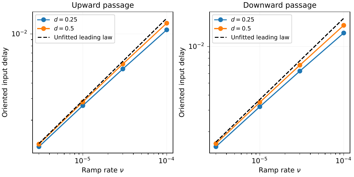
**[Figure 1](#figure-1). Source-derived delay scaling.** The two finite projection thresholds differ at each rate. Dashed curves use the fixed coefficients of [Table 1](/source-readout/slow-passage/02-folds-and-critical-coordinate#table-1) and are not fitted to the events.
The delay has the predicted orientation at both folds. At the slowest rate the actual-to-leading ratios for $d=0.25$ are about 0.943 upward and 0.915 downward. For $d=0.50$ they are about 0.988 and 0.969. The discrepancies decrease as the rate falls in the declared set. Log-delay fits against log rate give exponents between about 0.613 and 0.644, depending on fold and threshold. These finite-regime diagnostics retain subleading effects; the exponent and prefactor come from [Theorem 5.1](/source-readout/slow-passage/03-airy-delay-and-observables#theorem-5-1), not those fits.
### 10.2 Preparation, complete-state controls and independent formulation
At $\nu=3\times10^{-6}$, two additional outward runs start at the exact complete fold states and move outward through input distance $0.035$. Compare their events with [(47)](/source-readout/slow-passage/03-airy-delay-and-observables#eq-47) and the tracked-branch prediction. A smaller delay here comes from preparation, with no change to the fold location or memory law.
**[Table 5](#table-5). Exact-fold preparation at the slowest rate.** Ratio uses the preparation-specific leading coefficient with $\zeta_0$. The final column uses the tracked-branch coefficient with $\zeta_1$. Both are predictions from the source, without fitting.
| Fold | $d$ | $\Delta a$ | Fold-start lead | Ratio | Tracked lead |
| --- | ---: | ---: | ---: | ---: | ---: |
| Up | 0.25 | 0.0010298 | 0.0010990 | 0.93703 | 0.0012936 |
| Up | 0.50 | 0.0010884 | 0.0010990 | 0.99035 | 0.0012936 |
| Down | 0.25 | 0.0012635 | 0.0013988 | 0.90331 | 0.0016465 |
| Down | 0.50 | 0.0013536 | 0.0013988 | 0.96768 | 0.0016465 |
The transverse-preparation control adds all of the following to the initial low state of the slowest full cycle:
$$
\begin{aligned}
\delta(\Re z)&=(0.002,-0.001,0.0015),\\
\delta(\Im z)&=(-0.0015,0.001,0.0005),\\
\delta m&=(0.001,-0.0015).
\end{aligned}
\tag{66}
$$
This perturbs collective, reflection-odd, phase and memory directions before the long stable approach. Event changes are unresolved at the demonstrated integration accuracy. It does not test immunity to kicks inside the fold layer or to noise.
The uniqueness control changes only $\mu$ to 0.4 on the fastest identical triangle. Because $\mu>3\chi$, $\nabla^2V_{\rm eff}\ge(\mu-3\chi)I$ and strict stationary-memory convexity give a single equilibrium. Both memories still evolve in this adaptive control. The fixed-carrier control instead holds $K_0=\mu I+L$ and solves the same driven linear amplitude equation exactly. On each affine input segment, $k=\mu+3$, the slope is $v=\dot a$, and the initial modal amplitude is $u_0$:
$$
u(t)=\frac{a(t)}{ck}-\frac{v}{(ck)^2}+
\left(u_0-\frac{a(0)}{ck}+\frac{v}{(ck)^2}\right)e^{-ckt}.
\tag{67}
$$
The two control areas in [Table 6](#table-6) distinguish ordinary finite-rate lag in linear or single-state cases from the bistable cycle.
For an exactly symmetric preparation, ordinary reflection and zero collective amplitude give the invariant subspace $z=uv_3,\ m_1=m_2=m$. Its exact dynamical equations are
$$
\dot u=-c(\mu+3e^m)u+a(t),\qquad
\dot m=-\eta\left[\kappa m+\tfrac34e^m|u|^2\right].
\tag{68}
$$
A separately coded three-real-coordinate BDF integration of [(68)](#eq-68) uses relative tolerance $10^{-11}$, absolute tolerance $10^{-13}$ and half the primary step cap. It retains dynamic memory and compares all four slowest-cycle events with the complete Radau run. The symmetry restriction is exact for the symmetric preparation only. The complete-coordinate perturbation is a different experiment. Both solvers use SciPy; this is an independent formulation, not a second-platform replay.
**[Table 6](#table-6). Quality and control diagnostics.** The fixed and uniqueness-control areas are magnitudes of sampled oriented integrals. Event refinement, the modal comparison, and perturbation comparisons test different things. Small discrepancies do not give directed-arithmetic trajectory certificates.
| Check | Value |
| --- | ---: |
| Maximum event refinement difference | $3.730\times10^{-14}$ |
| Independent modal BDF difference | $3.840\times10^{-12}$ |
| Full Jacobian finite-difference error | $1.042\times10^{-9}$ |
| Initial perturbation event difference | $3.109\times10^{-15}$ |
| Fixed-carrier sampled area | $1.394\times10^{-6}$ |
| Unique adaptive sampled area | $4.569\times10^{-5}$ |
### 10.3 Continuous cycles, capture and work
The complete-state turn and return errors in [Table 7](#table-7) compare with the high stationary state at the reversal and the low stationary state at the return. These quantify capture and finite-rate lag. No finite-rate cycle is claimed to close exactly.
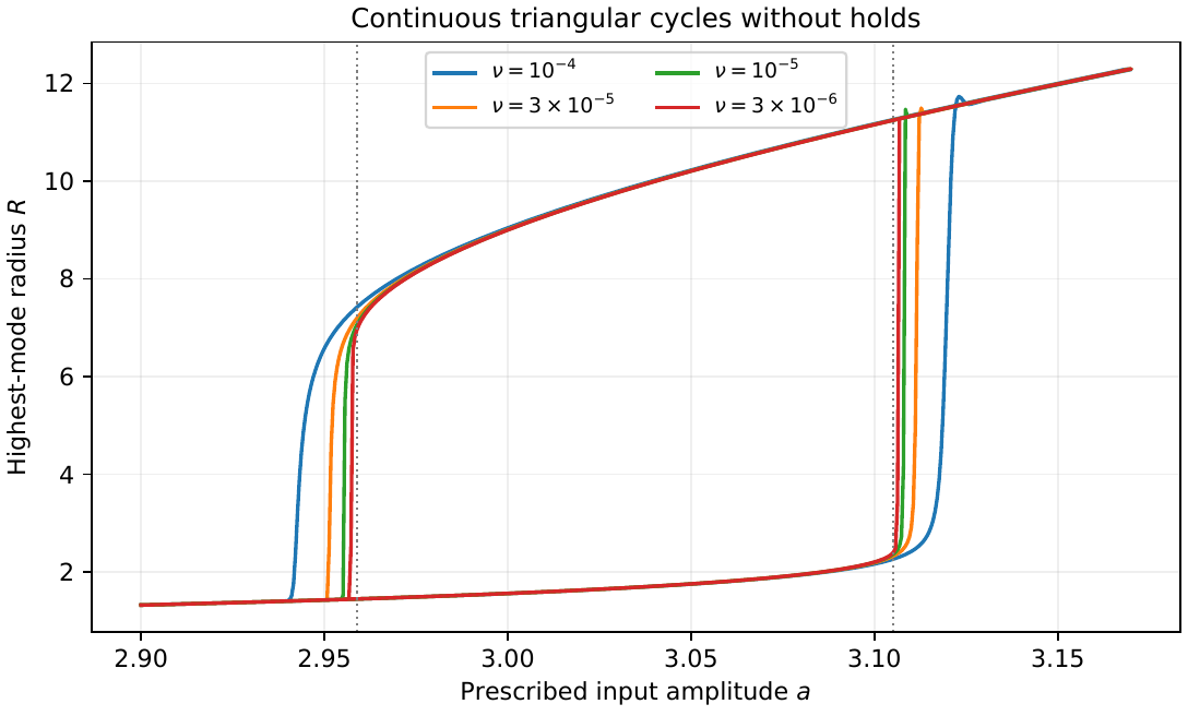
**[Figure 2](#figure-2). Complete-source trajectories at every declared rate.** Dotted lines mark static folds. Radius is sampled for display; switching inputs in Tables 3–4 come from independent event localization. Transient overshoot is allowed.
**[Table 7](#table-7). Capture, geometry and scaled work.** Turn and return errors are against $x_H(3.17)$ and $x_L(2.9)$. The sampled area evaluates [(55)](/source-readout/slow-passage/04-capture-hysteresis-and-work#eq-55) by trapezoids on the declared grid.
| Rate $\nu$ | Turn error | Return error | Sampled area | $\nu W$ |
| ---: | ---: | ---: | ---: | ---: |
| $1\times10^{-4}$ | $1.296\times10^{-2}$ | $8.541\times10^{-4}$ | 1.376522 | 1.65917591 |
| $3\times10^{-5}$ | $3.880\times10^{-3}$ | $2.557\times10^{-4}$ | 1.255423 | 1.65913088 |
| $1\times10^{-5}$ | $1.293\times10^{-3}$ | $8.520\times10^{-5}$ | 1.204922 | 1.65911939 |
| $3\times10^{-6}$ | $3.877\times10^{-4}$ | $2.556\times10^{-5}$ | 1.180157 | 1.65911558 |
**[Table 8](#table-8). Physical balances for each round trip.** $W$ is supplied work, $Q$ is dissipation and $\Delta F$ is the stored-energy change. The ledger ratio is the maximum per-leg physical or tilted residual normalized by $1+|W(t)|+|Q(t)|$.
| Rate $\nu$ | $W$ | $Q$ | $\Delta F$ | Ledger ratio |
| ---: | ---: | ---: | ---: | ---: |
| $1\times10^{-4}$ | 16591.75915 | 16591.75789 | $1.260\times10^{-3}$ | $1.48\times10^{-15}$ |
| $3\times10^{-5}$ | 55304.36251 | 55304.36213 | $3.772\times10^{-4}$ | $2.62\times10^{-15}$ |
| $1\times10^{-5}$ | 165911.93921 | 165911.93909 | $1.257\times10^{-4}$ | $2.65\times10^{-15}$ |
| $3\times10^{-6}$ | 553038.52752 | 553038.52749 | $3.769\times10^{-5}$ | $1.23\times10^{-15}$ |
Stationary-root quadrature gives $A_0\simeq1.15880536$ for [(56)](/source-readout/slow-passage/04-capture-hysteresis-and-work#eq-56). Finite-rate areas approach this value, without a certified trapezoidal area enclosure. The work coefficient from [(61)](/source-readout/slow-passage/04-capture-hysteresis-and-work#eq-61) is $C_W=1.659114$ in normalized units. The slowest computed $\nu W$ differs by less than $10^{-6}$ relative to that coefficient.
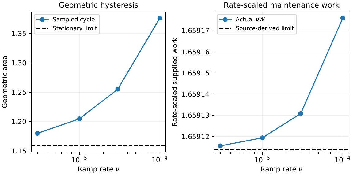
**[Figure 3](#figure-3). Geometry and energy have different limits.** Left: magnitude of the sampled oriented loop integral and the stationary-branch limit. Right: $\nu W$ and the source-derived work coefficient. The area remains finite while maintenance work grows like $1/\nu$. Neither panel claims a minimum switching work or identifies geometric area with physical energy.
### 10.4 Verification and correction traceability
The frozen criteria are $2\times10^{-8}$ for switching-input refinement and independent modal event differences, $2\times10^{-6}$ for refined endpoint differences, $2\times10^{-9}$ for scaled ledger errors, and $2\times10^{-7}$ for the early-preparation event comparison. Relative errors against the leading law have thresholds 0.35 at larger rates and 0.20 at the smallest rate. These finite-regime criteria were set before the ramp outputs. They are not constants in the asymptotic theorem.
All 113 frozen comparisons passed in the reported execution. Each fold has one zero mode and seven stable modes. Central finite differences at step $10^{-6}$ check the analytic Jacobian for the source and ledgers. Reflection equivariance is checked separately.
The public verification archive supplies code, settings, raw and checked outputs, correction records and generated assets. From the extracted archive, run the following with a new empty output directory:
~~~sh
python run_all.py --output ../new_replay
~~~
The runner repeats the full source, refinements, separate modal BDF calculation, local Jacobian checks and asset generation. It compares all 24 trajectory arrays with relative tolerance $2\times10^{-7}$ and absolute tolerance $2\times10^{-9}$. It reconstructs physical and tilted balances over whole cycles and validates the tables against the output of the same run. Eight checker regressions reject mutations of thresholds, event values, stable counts, labels and pass flags. They accept scientifically admissible diagnostic differences and irrelevant CSV line endings. Adaptive-step counts are incidental. Generated tables and figures are bound to that run's checked data and inputs.
Four archived raw exact-fold residuals require the reporting correction in Appendix A. The primary output formed those differences before replacing the tracked-initialization reference with the exact-fold reference. The correction recomputes only the four derived differences. It leaves switching inputs, prediction fields, leading ratios and all 113 comparison outcomes unchanged. The raw output is retained, each replay applies the correction, and the publication tables use checked values.
The documented run used Windows, Python 3.12.14, NumPy 2.3.5 and SciPy 1.18.1. The archive README provides dependency and execution instructions; VERIFICATION_RESULTS.json records the executed checks. Proofs establish the existence and asymptotic results under their hypotheses. Computation tests the finite-rate events and energy balances.
## What the Prepared Return Proves
## 11. Discussion
The static folds produce delayed switching through a mixed amplitude and memory direction. Complete left and right normalization fixes both load and quadratic coefficients, and therefore the prefactor of the two-thirds-power law. Preparation selects the Airy solution. A long stable approach and an exact-fold start remain distinct contracts even in the slow limit.
The local warrant is the invariant graph for seven complementary directions, with a finite-chart contraction estimate and parameter motion. The global warrant is strict loss at the fixed fold, supplying a complete connection, followed by continuity and regular tracking on the ramp. Neither substitutes stationary memory or assumes constant-input monotonicity during a sweep.
The prepared legs select different branches across coexistence, converge away from folds, and have the proved local input offsets and positive area limit. They can overshoot and do not prescribe an exact vertical trace. Fixed-rate attraction to a periodic response remains a separate question.
All declared rates and both numerical levels support the leading prediction, with preparation, symmetry and measurement controls. The levels have no certified chart radius. Explicit full-source finite-rate constants, higher-order terms, calibrated amplitude events, shrinking-neighborhood arrival, periodic-orbit attraction, noise and physical implementation remain open. A fitted log slope would not resolve them.
Equal stationary branch power fixes the leading work coefficient while memory changes the state and passage time. Slower traversal reduces switching-input displacement while increasing accumulated supplied work. Geometric hysteresis does not measure this work. Conditional coherent and dissipative linkage remains tied to one carrier; complete response retains source state and history. This finite constitutive mechanism extends maintained-state dynamics without claiming a common microscopic origin of unrelated spectral profiles.
## Appendix A. Finite-preparation residual audit
For exact-fold preparation define
$$
E_{\rm quad}=\Delta a_{\rm actual}-h_\nu T_d(k=1/\sqrt3).\tag{69}
$$
The four original derived fields instead subtracted $h_\nu T_d(k=0)$, the tracked-branch comparison, even though their stored predictions had been updated to the correct preparation. The checked output preserves the event locations, preparation-specific predictions, leading ratios and frozen comparison results. It changes a reporting difference rather than an experiment or tolerance.
| Fold | $d$ | Retained raw residual | Checked residual |
| --- | ---: | ---: | ---: |
| up | 0.25 | $-1.755594\times10^{-4}$ | $1.931485\times10^{-5}$ |
| up | 0.50 | $-1.604588\times10^{-4}$ | $3.418759\times10^{-5}$ |
| down | 0.25 | $-2.235553\times10^{-4}$ | $2.509803\times10^{-5}$ |
| down | 0.50 | $-2.109648\times10^{-4}$ | $3.686897\times10^{-5}$ |
**[Table 9](#table-9).** The four preserved raw differences and their checked counterparts at $\nu=3\times10^{-6}$. The public correction record retains the raw hash and all old and new values. Its executable stage computes [(69)](#eq-69) from the actual run's events and predictions. Scientific source and comparison criteria are unchanged.
## References
- Jack Carr. *Applications of Centre Manifold Theory*. Applied Mathematical Sciences 35, Springer, 1981. [DOI](https://doi.org/10.1007/978-1-4612-5929-9).
- Jack Carr. “Center manifold.” *Scholarpedia* 1(12):1826, 2006. [DOI](https://doi.org/10.4249/scholarpedia.1826), [article](https://www.scholarpedia.org/article/Center_manifold).
- Robert M. Corless, Gaston H. Gonnet, D. E. G. Hare, David J. Jeffrey, and Donald E. Knuth. “On the Lambert W function.” *Advances in Computational Mathematics* 5:329–359, 1996. [DOI](https://doi.org/10.1007/BF02124750).
- J. P. LaSalle. *The Stability of Dynamical Systems*. CBMS-NSF Regional Conference Series in Applied Mathematics 25, SIAM, 1976. [DOI](https://doi.org/10.1137/1.9781611970432).
- NIST. [Digital Library of Mathematical Functions: Airy and Related Functions](https://dlmf.nist.gov/9), sections 9.2, 9.7 and 9.9, accessed November 2026.
- Jeremy Rodgers. *Adaptive Spectral Carriers: Time Ordering, Reciprocal Memory, and Linked Coherent–Dissipative Response*, 2026a. [DOI](https://doi.org/10.5281/zenodo.23924603).
- Jeremy Rodgers. *Sharp Uniqueness and Bistability in Driven Adaptive Spectral Carriers*, 2026b. [DOI](https://doi.org/10.5281/zenodo.23932350).
- Jeremy Rodgers. *The Canonical Spectral-Curvature Field: A Unified Operator Origin for Coherence, Dissipation, and Spectral Budgets*, 2026c. [DOI](https://doi.org/10.5281/zenodo.23899458).
- Jeremy Rodgers. *Source Readout Non-Equivalence: Descent and Equivariant Reconstruction Obstructions*, 2026d. [DOI](https://doi.org/10.5281/zenodo.21369967).
- Jeremy Rodgers. *Observable Quotients and Exact Projected Dynamics: Closure, Memory, Minimal Dynamical Completion, and Effective Field Operators*, 2026e. [DOI](https://doi.org/10.5281/zenodo.21371251).
- Jeremy Rodgers. *Sustained Adaptive Spectral States: Global Attraction, Nonlinear Gain, and Linked Coherent–Dissipative Response*, 2026f. [DOI](https://doi.org/10.5281/zenodo.23927855).
- Arjan van der Schaft and Dimitri Jeltsema. “Port-Hamiltonian Systems Theory: An Introductory Overview.” *Foundations and Trends in Systems and Control* 1(2–3):173–378, 2014. [DOI](https://doi.org/10.1561/2600000002).