# Sharp Uniqueness and Bistability in Driven Adaptive Spectral Carriers
A sharp curvature threshold gives uniqueness even at equality. Below it, the three-node realization exhibits bistability, with a complete stationary count in the stated transverse-convexity regime.
Jeremy Rodgers · 2026-11-03
DOI: https://doi.org/10.5281/zenodo.23932350
## The Same Drive Can Sustain Two Stable States
## 1. The uniqueness boundary
One constant input can sustain two different stable amplitudes, memories and probe responses in the same finite reciprocal carrier. No change of constitutive law, controller, reservoir, saturation, or external power contract is required. The sharp curvature constant is $\chi=(2-\sqrt3)e^{-\sqrt3}$. For any finite incidence network, $\mu\ge\chi\lVert L\rVert$ guarantees one globally attracting equilibrium for every constant complex input, including equality. On a three-node path the threshold $3\chi$ is exact. For $0<\mu<3\chi$ suitable highest-mode inputs give two fully stable states. In the counted range $\chi<\mu<3\chi$ and inside the fold interval, there are exactly two minima and one index-one saddle.
The programme advances from one positive operator for coherent and dissipative evolution, through reciprocal adaptive memory, to externally sustained states. The present result closes the endpoint of the preceding strict sufficient condition. The proof proceeds through four bridges: stationary memory elimination and a strict line-convexity argument at zero minimum curvature; complete stationary-state counting beyond a scalar symmetry sector; the full dynamical index from stationary curvature; and a full-state tilted barrier whose membership test is separate from physical supplied work. Both folds are nondegenerate saddle-nodes in the counted regime. Independent modal cubics retain all eight eigenvalues.
Two stable states can have identical mean, stationary power and clamped static norm while responding differently to a later probe. That obstruction applies to the declared coarse summary and probe class. Calibrated complete stationary amplitude can instead reconstruct memory, without permitting dynamical memory elimination away from stationarity. Exact scalar certificates and reproducible finite numerical experiments support the worked example. The finite pulse switches are not evidence of a physical implementation or a quasistatic hysteresis limit. Atomic, image and Kerr signatures are not new tests of this model.
## 2. The complete source and external energy contract
### 2.1 Constitutive equations and units
Take $z\in\mathbb C^n$ and dimensionless edge memories $m\in\mathbb R^p$, with real incidence vectors $b_e\in\mathbb R^n$:
$$
B_e=b_eb_e^T,\quad L=\sum_e B_e,\quad K(m)=\mu I+\sum_e e^{m_e}B_e,\qquad \mu>0.\tag{1}
$$
Use the fixed Euclidean amplitude metric and its realification for all vector and induced operator norms. Edge stiffness is normalized to one. Positive baseline weights $k_e$ are incorporated by replacing each $b_e$ by $\sqrt{k_e}b_e$ everywhere, including $L$ and the curvature bound. In particular $K(m)\ge\mu I$ even in collective modes.
$$
F(z,m)=\frac12z^*K(m)z+\frac{\kappa}{2}|m|^2,\qquad \kappa>0.\tag{2}
$$
$$
g_e=(F_m)_e=\kappa m_e+\frac12 e^{m_e}|b_e^Tz|^2.\tag{3}
$$
With $c=\gamma+i\alpha$ and $\gamma,\alpha,\eta>0$, the reciprocal source is
$$
\dot z=-cK(m)z+f,\qquad \dot m=-\eta g(z,m).\tag{4}
$$
Except in the declared pulse experiments, $f\in\mathbb C^n$ is constant. The same stored energy generates the amplitude and memory efforts. This is a constitutive assumption of the finite realization. For amplitude, energy and time units $A,E,T$, respectively, the units of $K,\kappa,f,\gamma$ and $\alpha$, and $\eta$ are $E/A^2,E,A/T,A^2/(ET)$, and $1/(ET)$, respectively. Reference scales $A_0,E_0,T_0$ define the dimensionless coordinates used in Hessian and numerical comparisons.
### 2.2 Power and the constant-input tilt
The rate flow $f$ pairs with effort $Kz$. The signed power and physical balance are
$$
P=\operatorname{Re}[(Kz)^*f],\qquad \dot F=-\gamma\lVert Kz\rVert^2-\eta |g|^2+P.\tag{5}
$$
The ideal actuator can supply or absorb power and lies outside the modeled source state; no finite actuator energy store is included. The reactive term contributes no work since $\operatorname{Re}[i\alpha\lVert Kz\rVert^2]=0$. This is the effort–flow convention of van der Schaft and Jeltsema (2014).
For constant input let $\ell=f/c$ and introduce a tilted potential:
$$
V(z,m)=F(z,m)-\operatorname{Re}(\ell^*z).\tag{6}
$$
Write $q=(\operatorname{Re}z,\operatorname{Im}z)$, $K_R=\operatorname{diag}(K,K)$, and
$$
J=\begin{pmatrix}0&-I\\ I&0\end{pmatrix},\quad G=\gamma I+\alpha J,\quad
D=\operatorname{diag}(G,\eta I_p),\quad x=(q,m).\tag{7}
$$
Then $\dot x=-D\nabla V$, $\operatorname{Sym}D=\operatorname{diag}(\gamma I,\eta I)>0$, and
$$
\dot V=-\gamma\lVert Kz-\ell\rVert^2-\eta|g|^2.\tag{8}
$$
The tilt is a Lyapunov function. Physical supplied work is given by [(5)](#eq-5), not by the difference of tilted barriers.
**[Proposition 2.1](#proposition-2-1) (Boundedness and stationary limit sets).** Every initial state at constant $f$ gives a bounded global forward solution. Its omega-limit set is stationary. If the stationary set is finite, each solution converges to one point. No nonstationary trajectory is recurrent at fixed input.
**Proof.** Young's inequality and $K\ge\mu I$ give
$$
V\ge\frac\mu4\lVert z\rVert^2+\frac\kappa2|m|^2-\frac{\lVert\ell\rVert^2}{\mu}.\tag{9}
$$
The initial $V$ sublevel is compact and invariant by [(8)](#eq-8). The smooth vector field is locally Lipschitz, so continuation on this compact set rules out finite-time escape. If an omega-limit point were nonstationary, the loss in [(8)](#eq-8) would be bounded below on a small ball around it. Bounded velocity on the compact set implies infinitely many visits to a smaller ball entail infinitely many disjoint positive-duration intervals in the larger ball, with a common lower bound on duration. Their cumulative loss contradicts the finite limit of $V$. The omega-limit set is the nonempty compact connected intersection of the nested compact connected closures of continuous forward tails. A connected subset of a finite stationary set is a single point. Recurrence to a nonstationary point would require recovering its initial $V$ after strict decrease, contrary to monotonicity. This is the finite-dimensional strict-dissipation argument behind the invariance principle (LaSalle, 1976). $\square$
A finite pulse schedule concatenates globally defined constant-input segments. State and physical $F$ are continuous at each jump; $V$ changes by $-\operatorname{Re}[(\ell_{\rm new}-\ell_{\rm old})^*z]$. There is no single fixed tilt for such a schedule.
## Sharp Curvature and Complete Dynamical Stability
## 3. Stationary reduction and endpoint uniqueness
### 3.1 Exact memory elimination and curvature
At fixed $z$ the tilt is strictly convex in each memory:
$$
(F_{mm})_{ee}=\kappa+\tfrac12 e^{m_e}|b_e^Tz|^2\ge\kappa.\tag{10}
$$
Its minimizing value is $m_e=-s_e$, with
$$
s_ee^{s_e}=\frac{|b_e^Tz|^2}{2\kappa},\qquad s_e=W_0\!\left(\frac{|b_e^Tz|^2}{2\kappa}\right)\ge0.\tag{11}
$$
Only the real nonnegative principal Lambert branch is used (Corless et al., 1996). Substitution gives
$$
V_{\rm eff}(z)=\tfrac\mu2\lVert z\rVert^2+\sum_e\kappa(s_e+\tfrac12s_e^2)-\operatorname{Re}(\ell^*z).\tag{12}
$$
Critical points lift bijectively by [(11)](#eq-11) to complete stationary points. The elimination is stationary. The evolution of memory away from stationarity remains in the source.
For the edge coordinate $d=b_e^Tz\in\mathbb R^2$ the gradient is $wd$, with $w=e^{-s}$. The tangential curvature is $w$, and the radial curvature follows by $ds/d|d|=2s/[(1+s)|d|]$, extended continuously to $d=0$:
$$
w\frac{1-s}{1+s}=-Q(s),\qquad Q(s)=e^{-s}\frac{s-1}{s+1}.\tag{13}
$$
$$
Q'(s)=e^{-s}\frac{3-s^2}{(1+s)^2},\qquad \chi=\max_{s\ge0}Q(s)=(2-\sqrt3)e^{-\sqrt3}.\tag{14}
$$
The unique maximizer is $\sqrt3$. In real amplitude coordinates,
$$
\nabla^2V_{\rm eff}\ge\mu I-\chi L_R,\qquad L_R=\operatorname{diag}(L,L).\tag{15}
$$
**[Theorem 3.1](#theorem-3-1) (Closed sufficient uniqueness condition).** For a finite real incidence network and positive $\kappa,\gamma,\alpha,\eta$, if
$$
\mu\ge\chi\lVert L\rVert,\qquad\mu>0,\tag{16}
$$
then every constant complex input gives one globally asymptotically stable complete equilibrium. At equality $V_{\rm eff}$ is strictly convex and coercive; uniform strong convexity and a general positive exponential rate do not follow.
**Proof.** Strict inequality gives strong convexity by [(15)](#eq-15). At equality, with $L\ne0$, restrict to any nonconstant line $z(t)=z_0+t\xi$. Set $d_e(t)=b_e^Tz(t)$, $\delta_e=b_e^T\xi$ and let $\phi_e$ be the corresponding edge potential. Its line second derivative is
$$
\mu\lVert\xi\rVert^2-\chi\sum_e|b_e^T\xi|^2+
\sum_e\bigl(d^2\phi_e(d_e(t))[\delta_e,\delta_e]+\chi|\delta_e|^2\bigr).\tag{17}
$$
The first group and every edge remainder are nonnegative. If the first group vanishes, some $\delta_e\ne0$ because $\mu>0$ and $\xi\ne0$. Its remainder vanishes only at $s_e=\sqrt3$ with a radial $\delta_e$. The former requires
$$
|d_e(0)+t\delta_e|^2=2\kappa\sqrt3 e^{\sqrt3}.\tag{18}
$$
This nonconstant quadratic equality holds at most twice. The line derivative is strictly increasing on every interval, which proves strict convexity. If $L=0$, the positive amplitude quadratic suffices. Bound [(9)](/source-readout/sharp-uniqueness/01-complete-driven-source#eq-9) remains coercive after minimizing in $m$. The unique critical point is the strict global minimum of $V_{\rm eff}$; it lifts to the unique strict global minimum of $V$ because the minimizing memory is unique. [Proposition 2.1](/source-readout/sharp-uniqueness/01-complete-driven-source#proposition-2-1) supplies attraction. Compact sublevels and positive definiteness of $V-V_*$ supply Lyapunov stability. $\square$
The path endpoint below can have a zero Hessian direction. Failure of [(16)](#eq-16) does not determine uniqueness at a specified input. For example, $f=0$ gives only $(0,0)$ for any $\mu>0$.
## 4. Full stability from stationary curvature
### 4.1 Return the eliminated memory
At a stationary point in coordinates $(q,m)$, the complete Hessian is
$$
H=\begin{pmatrix}K_R&B\\B^T&H_m\end{pmatrix},\quad
B_{:e}=e^{m_e}\operatorname{diag}(B_e,B_e)q,\quad
H_m=\operatorname{diag}_e(\kappa+\tfrac12 e^{m_e}|b_e^Tz|^2).\tag{19}
$$
$$
S=K_R-BH_m^{-1}B^T=\nabla^2V_{\rm eff}.\tag{20}
$$
$$
(\xi,\nu)^TH(\xi,\nu)=\xi^TS\xi+
(\nu+H_m^{-1}B^T\xi)^TH_m(\nu+H_m^{-1}B^T\xi).\tag{21}
$$
Thus $H$ has the negative and zero counts of $S$ plus $p$ additional positive directions. Positivity of the clamped $K$ alone cannot classify the complete system.
**[Lemma 4.1](#lemma-4-1) (Mobility–inertia correspondence).** For real symmetric $H$ and real $D$ with $\operatorname{Sym}D>0$, the open right- and left-half-plane counts of $A=-DH$ equal the negative and positive inertia of $H$, with algebraic multiplicities over $\mathbb C$. Zero is semisimple of multiplicity $\dim\ker H$. No nonzero imaginary eigenvalue exists.
**Proof.** $D$ is invertible and
$$
\operatorname{Sym}(D^{-1})=D^{-T}(\operatorname{Sym}D)D^{-1}>0.\tag{22}
$$
If $Av=i\omega v$, $v\ne0$, $\omega\in\mathbb R\setminus\{0\}$, then $Hv\ne0$ and
$$
(Hv)^*D(Hv)=-i\omega v^*Hv.\tag{23}
$$
The left has strictly positive real part and the right has zero real part, since $H$ is Hermitian. Also $\ker A=\ker H$. A zero Jordan chain $Aw=v_0\ne0$ with $Hv_0=0$ would require
$$
0=v_0^*Hw=-v_0^*D^{-1}v_0,\tag{24}
$$
contradicting [(22)](#eq-22). Now homotope $D_t=(1-t)I+tD$ for $0\le t\le1$. The symmetric part remains positive. The imaginary axis is excluded apart from zero, whose fixed algebraic multiplicity prevents any additional eigenvalue reaching it. Continuity of characteristic roots preserves both open-half-plane counts from $-H$ at $t=0$. $\square$
For [(4)](/source-readout/sharp-uniqueness/01-complete-driven-source#eq-4), the full linearization is $-DH$. Positive $H_*$ gives a Hurwitz Jacobian and local nonlinear exponential stability. With $\sigma=\min(\gamma,\eta)$, $h_*=\lambda_{\min}(H_*)$ and $E=v^TH_*v/2$ for the perturbation $v$,
$$
\dot E\le-2\sigma h_*E+O(E^{3/2}).\tag{25}
$$
For every $0
### 4.2 Varying mobility at fixed state
With $H$ fixed, changes in mobilities preserving $\operatorname{Sym}D>0$ can affect transient behavior, eigenvalues and rates without changing the index, stabilizing a negative Hessian direction, or crossing through Hopf. Holding the stationary state fixed as $c$ changes requires $f=c\ell$ with fixed $\ell$. Holding physical $f$ fixed instead changes $\ell=f/c$ and generally the equilibrium and $H$.
## An Exact Bistability Threshold on Three Nodes
## 5. Three-node path: exact count and threshold
### 5.1 Modes and scalar stationary law
For $b_1=(1,-1,0)^T$, $b_2=(0,1,-1)^T$ the orthonormal eigenbasis is
$$
v_0=\frac{(1,1,1)^T}{\sqrt3},\quad v_1=\frac{(1,0,-1)^T}{\sqrt2},\quad v_3=\frac{(1,-2,1)^T}{\sqrt6},\qquad Lv_\lambda=\lambda v_\lambda.\tag{26}
$$
For $f=av_\lambda$, $a>0$ and $\lambda\in\{1,3\}$, equal-memory stationary states have $z=uv_\lambda$, $m_1=m_2=-s$, and $|b_e^Tz|^2=\lambda|u|^2/2$. Thus
$$
R^2=|u|^2=\frac{4\kappa}{\lambda}se^s,\qquad u=\frac{a/c}{\mu+\lambda e^{-s}}.\tag{27}
$$
$$
\frac{a^2}{|c|^2}=H_\lambda(s):=\frac{4\kappa}{\lambda}se^s(\mu+\lambda e^{-s})^2.\tag{28}
$$
The input fixes phase through $a/c$. Signed reflection yields the low-mode sector, ordinary reflection the highest-mode sector, with zero collective stationary amplitude. Differentiation gives
$$
H_\lambda'(s)=\frac{4\kappa}{\lambda}(\mu+\lambda e^{-s})e^s(1+s)[\mu-\lambda Q(s)].\tag{29}
$$
If $\mu\ge\lambda\chi$, the law increases strictly from zero to infinity; equality permits one isolated flat point. If $0<\mu<\lambda\chi$, the two roots of $Q(s)=\mu/\lambda$ obey
$$
1
$$
a_{\rm down}=|c|\sqrt{H_\lambda(s_+)},\qquad
a_{\rm up}=|c|\sqrt{H_\lambda(s_-)}.\tag{31}
$$
The three monotonicity intervals give three distinct positive roots in the open interval, two distinct roots including a double root at either endpoint, and one outside the closed interval. At an equal-edge equilibrium, rotate the common phase to make amplitude real. The radial and tangential Schur operators are $\mu I-Q(s)L$ and $\mu I+e^{-s}L$:
$$
\mu,\quad\mu-Q,\quad\mu-3Q;\qquad \mu,\quad\mu+w,\quad\mu+3w,\qquad w=e^{-s}.\tag{32}
$$
The two collective quadratures decay, since the mean $\bar z=(z_1+z_2+z_3)/3$ obeys
$$
\dot{\bar z}=-c\mu\bar z+\bar f.\tag{33}
$$
### 5.2 Sector stability can miss a full instability
At a low-mode fold $Q=\mu$, the transverse highest-mode radial curvature is $-2\mu<0$. A retained exact example takes $\mu=0.01$, $\kappa=1$, $s=5$, $a=|c|\sqrt{H_1(5)}$. Here $Q(5)=\tfrac23e^{-5}$ and rational exponential bounds give $1/300
### 5.3 Complete count for highest-mode preparation
**[Theorem 5.1](#theorem-5-1) (Complete path bistability).** For $\chi<\mu<3\chi$ and $f=av_3$, $a>0$, [(27)](#eq-27)–[(28)](#eq-28) with $\lambda=3$ give all equilibria. The open fold interval contains two locally exponentially stable minima and one index-one saddle. Outside the closed interval there is one globally asymptotically stable equilibrium. Each colliding pair at an endpoint has one zero and seven decaying linear modes. Every constant-input trajectory converges to a stationary point in these finite regimes.
**Proof.** Write $z=tv_0+uv_3+hv_1$ with complex $t,u,h$. Edges and forcing do not see $t$; the collective quadratic forces $t=0$ at stationarity. Reflection of nodes 1 and 3 fixes $v_3$, reverses $v_1$, and interchanges edges up to irrelevant signs. At fixed $u$ the potential is even in $h$, and the $v_1$ eigenvalue of $L$ gives
$$
\nabla_h^2V_{\rm eff}\ge(\mu-\chi)I_2>0.\tag{34}
$$
Thus $h=0$ is its unique critical point. Both edge magnitudes then coincide, so [(11)](/source-readout/sharp-uniqueness/02-endpoint-and-stability#eq-11) gives $m_1=m_2=-s$. The stationary amplitude equation fixes $u=(a/c)/(\mu+3e^{-s})$, yielding exactly [(28)](#eq-28). The scalar count is therefore complete. Outer branches have $Q<\mu/3$; [(32)](#eq-32), [(21)](/source-readout/sharp-uniqueness/02-endpoint-and-stability#eq-21), and [Lemma 4.1](/source-readout/sharp-uniqueness/02-endpoint-and-stability#lemma-4-1) give local exponential stability. The middle branch has $\mu/3
**[Corollary 5.2](#corollary-5-2) (Sharp path threshold and optimal universal coefficient).** Every constant complex input on this path has exactly one globally asymptotically stable equilibrium if and only if $\mu\ge3\chi$. Consequently $\chi$ is the smallest universal sufficient coefficient $C$ in $\mu\ge C\lVert L\rVert$.
**Proof.** $\lVert L\rVert=3$, so [Theorem 3.1](/source-readout/sharp-uniqueness/02-endpoint-and-stability#theorem-3-1) gives sufficiency. For every $0<\mu<3\chi$, choose highest-mode load strictly between the folds. Both outer scalar roots obey $Q<\mu/3$ and are fully stable by [(32)](#eq-32) and [Lemma 4.1](/source-readout/sharp-uniqueness/02-endpoint-and-stability#lemma-4-1). This disproves all-input uniqueness even for $\mu\le\chi$, where the entire stationary set has not been counted. If $C<\chi$, choose positive $\mu<3\chi$ with $\mu\ge3C$ to disprove that universal coefficient. $\square$
These are distinct statements: a universal sufficient condition, its optimal coefficient over networks, an exact all-input threshold on one path, and uniqueness at one specified drive. At fixed physical $a$ the three-state condition in the counted range is exactly
$$
H_3(s_+)<\frac{a^2}{\gamma^2+\alpha^2}0$. At a positive endpoint the load derivative $-2\alpha a^2/(\gamma^2+\alpha^2)^2$ is nonzero, so mobility can pass through a fold at fixed physical drive. This changes the stationary Hessian and does not contradict the fixed-$H$ result. The stationary equations do not contain $\eta$.
## Both Folds Are Full Dynamical Saddle-Nodes
## 6. Saddle-nodes and complete modal cubics
### 6.1 Full dynamical nondegeneracy
A stationary turning point does not by itself establish a dynamical saddle-node. In the range of [Theorem 5.1](/source-readout/sharp-uniqueness/03-sharp-path-threshold#theorem-5-1) fix $c$ and write the stationary curve as
$$
R(s)=\sqrt{\tfrac{4\kappa}{3}se^s},\quad z(s)=\frac{|c|}{c}R(s)v_3,\quad
m(s)=(-s,-s),\quad a(s)=|c|\sqrt{H_3(s)}.\tag{36}
$$
In real coordinates $x(s)$ the stationary map and vector field are
$$
Y(x,a)=\nabla F(x)-ah,\quad h=(\operatorname{Re}(v_3/c),\operatorname{Im}(v_3/c),0,0),\quad X(x,a)=-DY(x,a).\tag{37}
$$
The order of $-D$ on the left matters. At a fold $a'=0$, differentiate $Y(x(s),a(s))=0$. Then $r=x'(s)$ spans $\ker H$ by [Theorem 5.1](/source-readout/sharp-uniqueness/03-sharp-path-threshold#theorem-5-1), and
$$
r^Th=R'(s)/|c|>0,\qquad d=r^TD^{-1}r>0.\tag{38}
$$
Thus $l^T=r^TD^{-1}/d$ is a normalized left null vector of $A=-DH$, with $l^Tr=1$. The normalization uses the actual derivative $r$, not a unit vector. The load coefficient is
$$
l^TX_a=\frac{r^Th}{d}>0.\tag{39}
$$
Differentiate the stationary identity twice and multiply by $r^T$ to obtain
$$
r^TY_{xx}[r,r]=(r^Th)a'',\qquad
\tfrac12 l^TX_{xx}[r,r]=-\frac{(r^Th)a''}{2d}.\tag{40}
$$
At a fold $a''=|c|H_3''/(2\sqrt{H_3})$ and
$$
H_3''(s)=\tfrac{4\kappa}{3}\bigl[\mu^2e^s(s+2)+9e^{-s}(s-2)\bigr].\tag{41}
$$
Equation [(29)](/source-readout/sharp-uniqueness/03-sharp-path-threshold#eq-29) shows the sign is opposite to $Q'$. Thus $a''<0$ at $s_-$ and $a''>0$ at $s_+$, with neither zero. The one simple zero, seven decaying modes, and nonzero load and quadratic terms give both full saddle-nodes by the usual conditions (Kuznetsov, 2004). The quadratic coefficient is positive at the upper-input fold and negative at the lower one.
At $\mu=3\chi$, $s=\sqrt3$, the scalar folds meet. Strict convexity still gives a unique equilibrium at the critical input, but the Jacobian has a zero eigenvalue. Neither linear exponential stability nor a general positive local exponential estimate follows there. A cusp claim would require additional higher-order and unfolding conditions.
### 6.2 Independent all-coordinate blocks
Rotate the common equilibrium phase to make $z$ real. The three orthonormal node modes and the memories $(\delta m_1\pm\delta m_2)/\sqrt2$ give an orthogonal transform of the eight-dimensional source. The collective pair is
$$
p=-\mu(\gamma\pm i\alpha).\tag{42}
$$
For $\lambda=1,3$ the Hessian and mobility blocks, with a chosen memory sign, are
$$
H_\lambda=\begin{pmatrix}k&0&\beta\\0&k&0\\\beta&0&h\end{pmatrix},\qquad
D_\lambda=\begin{pmatrix}\gamma&-\alpha&0\\\alpha&\gamma&0\\0&0&\eta\end{pmatrix}.\tag{43}
$$
$$
k=\mu+\lambda w,\quad h=\kappa(1+s),\quad \beta^2=2\kappa\lambda sw,\quad w=e^{-s}.\tag{44}
$$
For source mode $v_j$, $j\in\{1,3\}$, the coupling squared is $w^2R^2\sum_e(b_e^Tv_j)^2(b_e^Tv_\lambda)^2$. The sum is $j\lambda/2$ and $R^2=(4\kappa/j)se^s$, giving [(44)](#eq-44). Highest-mode drive pairs $\lambda=3$ with even memory and $\lambda=1$ with odd memory; low-mode drive reverses that assignment. Each block keeps radial and phase amplitude and one memory coordinate.
$$
\begin{aligned}
P_\lambda(p)&=(p^2+2\gamma kp+|c|^2k^2)(p+\eta h)-\eta\beta^2(\gamma p+|c|^2k)\\
&=p^3+A_2p^2+A_1p+A_0,\\
A_2&=2\gamma k+\eta h,\\
A_1&=|c|^2k^2+\eta\gamma(2hk-\beta^2),\\
A_0&=\eta|c|^2k(hk-\beta^2).
\end{aligned}\tag{45}
$$
$$
\rho=k-\beta^2/h=\mu-\lambda Q(s).\tag{46}
$$
Also $2hk-\beta^2=2\kappa[(1+s)\mu+\lambda w]>0$ and
$$
A_2A_1-A_0=2\gamma|c|^2k^3+\eta|c|^2k\beta^2+
\eta\gamma(2\gamma k+\eta h)(2hk-\beta^2)>0.\tag{47}
$$
Hence $A_2,A_1>0$. When $\rho>0$, vary $A_0$ from zero through $00$ for $p\ge0$ give exactly one positive real root. The remaining roots have positive product and negative sum, hence negative real parts. This elementary argument is independent of the general inertia proof.
The two cubics and the collective pair count all eight eigenvalues with multiplicity. Numerical roots of the cubics and direct matrix spectra test different formulations with a shared numerical eigensolver backend.
## Full-State Basins, Powered Switches and Lost Readout Information
## 7. Full-state basin regions and powered switching
### 7.1 A cylinder barrier
In the three-equilibrium regime write $x_L,x_M,x_H$ for low, middle and high, $V_M=V(x_M)$, $R_M=|v_3^Tz_M|$.
**[Theorem 7.1](#theorem-7-1) (Sufficient complete basin criterion).** Each complete initial state satisfying [(48)](#eq-48) converges to $x_L$; each satisfying [(49)](#eq-49) converges to $x_H$. The criteria allow arbitrary collective, odd, phase and memory disturbances within the stated inequalities.
$$
V(x)
$$
V(x)R_M.\tag{49}
$$
**Proof.** On any full state $V(z,m)\ge V_{\rm eff}(z)$. For fixed highest-mode coordinate $u$, the collective quadratic is minimized at $t=0$ and the strictly convex reflection-even odd slice at $h=0$. With $\theta=|c|/c$, the forcing term at fixed radius is minimized by phase alignment with $a/c$. On the cylinder $|v_3^Tz|=R_M$,
$$
V(z,m)\ge V_{\rm eff}(uv_3)\ge V_{\rm eff}(\theta R_Mv_3)=V_M.\tag{50}
$$
The first effective term uses the actual phase; the second minimizes it. The full strict sublevel is invariant, and continuity prevents crossing the cylinder. [Proposition 2.1](/source-readout/sharp-uniqueness/01-complete-driven-source#proposition-2-1) gives convergence to one of the three equilibria. The strict loss bound excludes the middle state, and only the target has radius on the correct side. $\square$
Both minima are below $V_M$. On the aligned ray write the potential as $W(R)$:
$$
W'(R)=(\mu+3e^{-s(R)})R-a/|c|.\tag{51}
$$
The derivative signs through the three simple roots are negative, positive, negative, positive. Integrating between roots gives $V_L,V_H
### 7.2 Finite pulse experiments and resources
A pulse across a fold, followed by restoration of the same base drive, can move a complete source into the other attraction basin. This is an executed numerical schedule, not a conclusion from the stationary diagram alone. The two directions were run independently, not as one cycle.
| Pulse | Initial state | $a_{\rm pulse}$ | $T_{\rm pulse}$ | $a_{\rm return}$ | $T_{\rm return}$ |
| --- | --- | ---: | ---: | ---: | ---: |
| up | low | 3.3 | 300 | 3.0 | 600 |
| down | high | 2.7 | 300 | 3.0 | 600 |
**[Table 1](#table-1).** Prescribed square pulses return to the identical $f=3v_3$. Times and amplitudes are normalized as in [Section 2](/source-readout/sharp-uniqueness/01-complete-driven-source#section-2).
$$
W_{\rm in}(T)=\int_0^T P\,dt,\qquad Q_{\rm diss}(T)=\int_0^T(\gamma\lVert Kz\rVert^2+\eta|g|^2)\,dt,\qquad \Delta F=W_{\rm in}-Q_{\rm diss}.\tag{52}
$$
At jumps the state and $F$ are continuous; $V$ changes by the input-dependent tilt. Monotonicity is used only within each constant segment. Each terminal state lies in the strict target barrier region at the restored input, with small numerical target-state error. These convergence-checked floating trajectories are not interval-flow certificates, minimum switching work, or a dynamic quasistatic limit.
At stationarity $Kz=f/c$ and $g=0$, so
$$
P_*=\gamma\frac{\lVert f\rVert^2}{|c|^2}>0\quad(f\ne0).\tag{53}
$$
Under convergence at fixed input $P(t)\to P_*$ and $W_{\rm in}(T)=P_*T+o(T)$. Stored energy converges and accumulated dissipation has the same leading growth. Both stable memories are powered open-system states. An unreplenished finite source cannot sustain either indefinitely under this contract.
## 8. Observable response and source-to-readout information
### 8.1 Conditional versus free memory
On an imposed memory history,
$$
\partial_tU(t,s)=-cK(m(t))U(t,s),\qquad U(s,s)=I,\qquad
z(t)=U(t,0)z(0)+\int_0^tU(t,s)f(s)\,ds.\tag{54}
$$
Instantaneous dissipative and coherent generators are $\gamma K$ and $\alpha K$, with fixed ratio $\alpha/\gamma$. The freely adapting Jacobian adds memory. For a small real amplitude-rate probe $r(t)$ at a stationary source,
$$
\dot\xi=-GK_R\xi-GB\nu+r,\qquad \dot\nu=-\eta B^T\xi-\eta H_m\nu.\tag{55}
$$
Exact dynamical elimination keeps both initial memory and causal history:
$$
\dot\xi(t)=-GK_R\xi(t)-GBe^{-\eta H_mt}\nu(0)+r(t)
+\eta\int_0^tGBe^{-\eta H_m(t-s)}B^T\xi(s)\,ds.\tag{56}
$$
The factors cannot be commuted. With zero initial perturbation,
$$
\chi_{\rm full}(p)^{-1}=pI+GK_R-\eta GB(pI+\eta H_m)^{-1}B^T.\tag{57}
$$
Clamping gives $\chi_{\rm clamp}(p)=(pI+GK_R)^{-1}$. At the minima $A$ is Hurwitz and $H_m>0$, so block Schur inversion of $pI-A$ gives invertibility of [(57)](#eq-57) for $\operatorname{Re}p\ge0$ and a stable causal response. The static equation is $GS\xi=r$:
$$
\chi_{\rm full}(0)=S^{-1}G^{-1},\qquad \chi_{\rm clamp}(0)=K_R^{-1}G^{-1}.\tag{58}
$$
At the saddle the full static formula is an algebraic derivative, not a stable susceptibility. The simple positive eigenvalue is visible in the amplitude transfer: either its right or its left eigenvector having zero amplitude component would force the eigenvalue to belong to $-\eta H_m$, which is negative definite. At folds $S$ is singular so even the algebraic inverse fails. The clamped amplitude remains stable everywhere here because $K>0$; this says nothing about full source stability.
### 8.2 What the coarse summary loses
With a collective mode the smallest eigenvalue of $K$ is $\mu$; $|c|G^{-1}$ is orthogonal. Therefore, for nonsingular $S$,
$$
\lVert\chi_{\rm clamp}(0)\rVert=\frac1{|c|\mu},\qquad
\lVert S^{-1}G^{-1}\rVert=\frac1{|c|\min_j|\lambda_j(S)|}.\tag{59}
$$
$$
O(x_*)=(\bar z_*,P_*,\lVert\chi_{\rm clamp}(0)\rVert).\tag{60}
$$
Both stable states of the worked example share $O=(0,3,1/(|c|\mu))$, but their full static norms differ. The full operators differ, so some common small phase-sensitive amplitude-rate probe has different stationary linear responses under free memory. The coarse summary cannot predict every such continuation. That claim uses calibrated additive probes, phase-sensitive access, and a distinction between free and clamped memory; it does not extend to arbitrary unadmitted operations.
The loss is readout-specific (Rodgers, 2026c,d). Full calibrated stationary $z$ determines each memory by [(11)](/source-readout/sharp-uniqueness/02-endpoint-and-stability#eq-11), whereas instantaneous nonstationary $z(t)$ does not determine independent $m(t)$. Stationary reconstruction does not erase the kernel in [(56)](#eq-56). The two maintained states differ in amplitude, stored energy, memory, edge weight and free response. Their conditional coherent and dissipative edge stiffnesses change together. Equal supplied power reflects equal actuator norm, not equality of state or response.
## The Three-Node Example in Numbers
## 9. Fixed example and numerical evidence
### 9.1 Analytic design and stationary values
$$
(\mu,\kappa,\gamma,\alpha,\eta)=(0.1,1,0.6,1.2,0.8),\qquad f=3v_3.\tag{61}
$$
Here $\chi\simeq0.04740589436$, $\chi<\mu<3\chi$, and $\mu-3\chi<0$. The load $a^2/|c|^2$ is exactly 5 and
$$
H_3(s)=\tfrac1{75}se^s+\tfrac45s+12se^{-s}.\tag{62}
$$
Order-40 rational Taylor bounds with geometric tails show $H_3(0)<5
| Branch | $s$ | $R$ | $F$ | $V$ | $n_+$ |
| --- | ---: | ---: | ---: | ---: | ---: |
| low | 0.811988 | 1.561583 | 2.405227 | -1.086579 | 0 |
| middle | 2.088707 | 4.742040 | 9.664461 | -0.939063 | 1 |
| high | 3.006220 | 9.000611 | 19.100345 | -1.025633 | 0 |
**[Table 2](#table-2).** $R=\lVert z_*\rVert$, $m_1=m_2=-s$. The two outer states have eight decaying modes; the middle has seven decaying modes and one unstable eigenvalue.
| Branch | $e^{-s}$ | $P_*$ | $\lVert\chi_{\rm clamp}\rVert$ | $\lVert\chi_{\rm full}\rVert$ |
| --- | ---: | ---: | ---: | ---: |
| low | 0.443975 | 3.000000 | 7.453560 | 7.453560 |
| middle | 0.123847 | 3.000000 | 7.453560 | 24.074130 |
| high | 0.049478 | 3.000000 | 7.453560 | 29.039222 |
**[Table 3](#table-3).** Edge weight, stationary power and static norms. All means vanish. The middle full entry is an algebraic derivative; the outer entries are stable full-feedback responses.
| Fold | $s$ | $a$ | $l^TX_a$ | $\tfrac12l^TX_{xx}[r,r]$ |
| --- | ---: | ---: | ---: | ---: |
| Upper input | 1.269082 | 3.105014 | 0.398392 | 0.133396 |
| Lower input | 2.585036 | 2.958897 | 0.355600 | -0.072477 |
**[Table 4](#table-4).** Complete dynamical coefficients with $r=x'(s)$ and $l^Tr=1$. The upper input is at the smaller $s$; both coefficients are bounded away from zero in the numerical checks.
The high-amplitude branch has more negative memory, weaker edge stiffness and greater stored energy, yet its tilted minimum is not the lower one. Equal power and clamped norm coexist with distinct full responses. The base drive is strictly between the two folds.
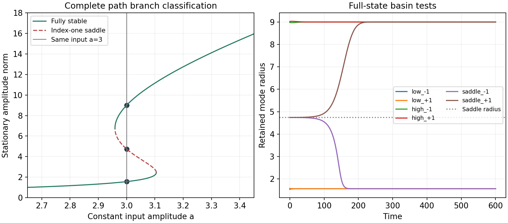
**[Figure 1](#figure-1).** Left: sampled exact branch law and proved full stability classification at the common base input. Right: full-state basin preparations. The saddle radius is a barrier only together with the tilted-energy condition.
### 9.2 Full-state preparations and controls
Use real coordinate order $(\operatorname{Re}z_1,\operatorname{Re}z_2,\operatorname{Re}z_3,\operatorname{Im}z_1,\operatorname{Im}z_2,\operatorname{Im}z_3,m_1,m_2)$. Four starts add or subtract
$$
d=(0.02,-0.01,0.015,-0.015,0.01,0.005,0.01,-0.015)\tag{63}
$$
from the low or high state. Two add or subtract $0.001$ times the middle state's normalized real unstable vector, oriented toward increasing $R$. These are full-coordinate perturbations and all satisfy the proper barrier conditions.
| Preparation | Target | $V_M-V(0)$ | Final error | Ledger error |
| --- | --- | ---: | ---: | ---: |
| `low_-1` | low | 1.466e-01 | 3.48e-14 | 3.02e-11 |
| `low_+1` | low | 1.466e-01 | 3.53e-14 | 2.89e-11 |
| `high_-1` | high | 8.575e-02 | 1.04e-13 | 8.07e-11 |
| `high_+1` | high | 8.574e-02 | 1.06e-13 | 4.18e-11 |
| `saddle_-1` | low | 1.217e-08 | 2.80e-14 | 1.94e-09 |
| `saddle_+1` | high | 1.216e-08 | 1.63e-13 | 1.11e-09 |
**[Table 5](#table-5).** Six complete trajectories to $T=600$. Final error is Euclidean full-state distance to target; ledger error is the maximum sampled absolute physical balance residual. Diagnostic digits are not acceptance thresholds.
The fixed-carrier control sets $m=0$, $K_0=\mu I+L$, keeps the drive, and starts from the amplitude of either unperturbed adaptive outer state. The exact matrix exponential converges in both cases to $z_{\rm fixed}^*=f/[c(\mu+3)]$, norm $\sqrt5/3.1$. The second control changes only $\mu$ to $0.4>3\chi$, starts at the main high equilibrium plus $d$, and converges to the unique state guaranteed by [Theorem 3.1](/source-readout/sharp-uniqueness/02-endpoint-and-stability#theorem-3-1).
| Control | Quantity | Value |
| --- | --- | ---: |
| Fixed carrier | Stored energy | 0.806452 |
| Fixed carrier | Stationary power | 3 |
| Unique adaptive | $\mu$ | 0.4 |
| Unique adaptive | Final error | 2.75885e-15 |
| Real-gradient RK4 | Difference | 3.41061e-13 |
**[Table 6](#table-6).** The fixed-carrier power agrees with the adaptive states although energy and amplitude differ. The RK4 difference compares states and physical ledgers in the separate $T=60$ run.
### 9.3 Physical ledgers for the two switches
Each 300-unit pulse precedes 600 units at the restored base input. Upward and downward terminal states enter the high and low strict barrier regions, respectively. Target errors are below $4\times10^{-13}$ and physical balance residuals below $2\times10^{-9}$. The cumulative work mostly maintains the driven state and is not the tilted barrier.
| Pulse | Work | Dissipation | $\Delta F$ | Final margin |
| --- | ---: | ---: | ---: | ---: |
| up | 2900.664693 | 2883.969575 | 16.695118 | 0.086570 |
| down | 2520.086406 | 2536.781523 | -16.695118 | 0.147515 |
**[Table 7](#table-7).** Work and dissipation at $T=900$. Final margin is $V_M-V(x(T))$ at restored drive. Opposite energy changes reflect different endpoints, while both runs require positive supplied work.
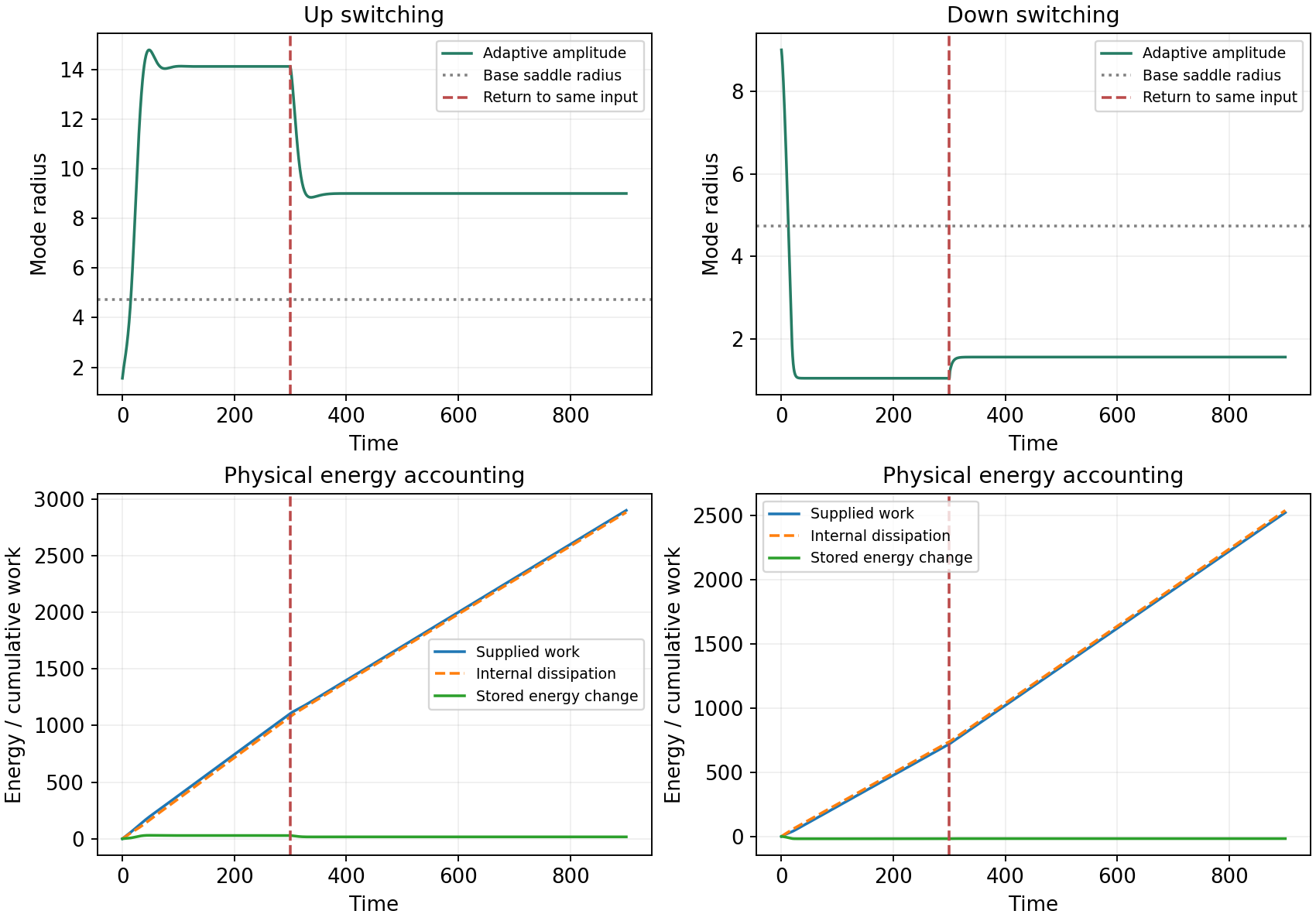
**[Figure 2](#figure-2).** Dashed vertical lines mark return to the same input. Cumulative work minus dissipation equals the stored-energy change within numerical tolerance. No slow sweep is executed in these experiments.
### 9.4 Methods and reproduction
Primary DOP853 relative and absolute tolerances are $10^{-10}$ and $10^{-12}$, with separate solves at input jumps. Each run is repeated at $10^{-12}$ and $10^{-14}$. The maximum step follows the source scale:
$$
\Delta t_{\max}=\frac1{8|c|[\mu+e^{M_0}\lVert L\rVert]},\qquad M_0=\max(0,\max_e m_e(0)).\tag{64}
$$
When $m_e\ge0$, $\dot m_e\le-\eta\kappa m_e$, so $m_e(t)\le\max(0,m_e(0))$ and $K(t)\le\mu I+e^{M_0}L$. This caps the carrier scale, not the error by a rigorous enclosure. Basins store 1,201 times over $T=600$; pulse segments each store 601 with the common endpoint retained once. Work and dissipation are integrated as extra variables.
Scalar roots are bracketed at absolute tolerance $10^{-13}$. Direct eight-coordinate stationary solves use the full Hessian, with independent scalar comparisons. Check the full Schur spectrum against [(32)](/source-readout/sharp-uniqueness/03-sharp-path-threshold#eq-32), central-difference the full vector field at step $10^{-5}$, and compute fold second differences at $10^{-4}$. Retained ceilings are $10^{-9}$ for stationary and Schur residuals, $2\times10^{-6}$ for Jacobian differences, $2\times10^{-5}$ for fold differences and $2\times10^{-7}$ for trajectory and ledger errors. Fold transversality and quadratic magnitudes must exceed $10^{-6}$; zero-eigenvalue tolerance is $10^{-7}$.
Independent scalar checks use 70-digit Decimal exponentials and 220 bisections without SciPy or Lambert W. Fraction arithmetic checks order-40 scalar bounds, including the rejected low-mode candidate. Real-gradient RK4 separately integrates eight coordinates and two ledgers for $T=60$, step $0.002$, and agrees with tight DOP853 within $2\times10^{-7}$. This does not replay the full switching schedule independently. Six modal fixtures compare cubics plus collective pair to complete matrices for all branches, folds and the negative candidate. The maximum observed spectral difference is below $6\times10^{-15}$ with shared NumPy eigensolver. Fixed-H fixtures set $\alpha=0.12,1.2,12$ and adjust $f=c\ell$; the endpoint has one zero and no unstable eigenvalue.
The public runner checks 114 numerical conditions, 20 arrays at relative $2\times10^{-8}$ and absolute $2\times10^{-10}$, six cubic fixtures, and tables generated in the replay. Eight checker regressions reject changed scientific thresholds, counts, labels, states and flags, while allowing sub-ceiling diagnostics and irrelevant line endings. Spectra are matched as multisets. A saved-identity audit checks fixed-carrier endpoint, physical balance and response formulas; it is a post-result algebraic audit rather than a fresh holdout.
The package includes the inputs, specifications, code, dependencies, reference outputs, hashes, own-run table generation and clean-extraction instructions. Proofs establish general and complete-count statements; exact bounds certify scalar claims; floating matrices and trajectories evaluate the example. Independent formulations and same-code replay serve different verification roles. No fresh dependency installation, certified flow enclosure or physical experiment is claimed by the paper.
## What the Threshold and Readout Obstruction Establish
## 10. Discussion and limits
The sharp threshold compares baseline stiffness with the most negative stationary edge curvature. Excitation weakens an edge; the quadratic memory cost bounds the curvature loss. At and above $\mu=\chi\lVert L\rVert$ strict convexity selects one full stationary source at every constant drive. Below the path threshold two stable states can persist at the same drive, separated by a saddle in the counted regime. The full Hessian governs their survival under arbitrary perturbations.
Highest-mode forcing aligns explicit scalar reduction with global exclusion of reflection-broken equilibria when $\mu>\chi$. The memory lift and inertia lemma restore all coordinates. The low-mode failure shows why the return matters. At $\mu\le\chi$ the two outer high-mode roots still disprove uniqueness, but additional roots have not been completely counted. Individual networks below the universal bound need separate geometry.
Complete saddle-nodes rely on the stated nondegeneracy conditions. Reactive mobility preserves inertia at fixed Hessian yet changes stationary load at fixed physical input. A comparison must specify which it holds fixed. Memory clamping also changes the experiment: conditional linked generators survive while free memory adds a causal kernel and changes static gain.
The barrier regions are sufficient, not a complete description of the saddle stable set. The numerical square pulses switch at finite time and return to identical input with explicit energy ledgers. They do not prove a quasistatic limit, minimum work, noisy retention, or experimental realization. A physical implementation needs calibrated reciprocal constitutive behavior, controlled drive, phase-sensitive access and a justified free-versus-clamped probe protocol.
Identical coarse present data can fail to determine the admitted future response; richer calibrated stationary amplitude can recover memory. Continuous external power sustains both alternatives. This is a complete constitutive mechanism in the counted regime, not a common microscopic explanation of different spectral domains. For slowly swept inputs, continue to [Slow Passage and Prepared Hysteresis](/source-readout/slow-passage).
## References
- Robert M. Corless, Gaston H. Gonnet, D. E. G. Hare, David J. Jeffrey, and Donald E. Knuth. “On the Lambert W function.” *Advances in Computational Mathematics* 5:329–359, 1996. [DOI](https://doi.org/10.1007/BF02124750).
- Yuri A. Kuznetsov. *Elements of Applied Bifurcation Theory*. Applied Mathematical Sciences 112, 3rd ed., Springer, 2004. [DOI](https://doi.org/10.1007/978-1-4757-3978-7).
- J. P. LaSalle. *The Stability of Dynamical Systems*. CBMS-NSF Regional Conference Series in Applied Mathematics 25, SIAM, 1976. [DOI](https://doi.org/10.1137/1.9781611970432).
- Jeremy Rodgers. *Adaptive Spectral Carriers: Time Ordering, Reciprocal Memory, and Linked Coherent–Dissipative Response*, 2026a. [DOI](https://doi.org/10.5281/zenodo.23924603).
- Jeremy Rodgers. *The Canonical Spectral-Curvature Field: A Unified Operator Origin for Coherence, Dissipation, and Spectral Budgets*, 2026b. [DOI](https://doi.org/10.5281/zenodo.23899458).
- Jeremy Rodgers. *Source Readout Non-Equivalence: Descent and Equivariant Reconstruction Obstructions*, 2026c. [DOI](https://doi.org/10.5281/zenodo.21369967).
- Jeremy Rodgers. *Observable Quotients and Exact Projected Dynamics: Closure, Memory, Minimal Dynamical Completion, and Effective Field Operators*, 2026d. [DOI](https://doi.org/10.5281/zenodo.21371251).
- Jeremy Rodgers. *Sustained Adaptive Spectral States: Global Attraction, Nonlinear Gain, and Linked Coherent–Dissipative Response*, 2026e. [DOI](https://doi.org/10.5281/zenodo.23927855).
- Arjan van der Schaft and D. Jeltsema. *Port-Hamiltonian Systems Theory: An Introductory Overview*. *Foundations and Trends in Systems and Control* 1, nos. 2–3, Now Publishers, 2014. [DOI](https://doi.org/10.1561/2600000002).