# The Canonical Spectral-Curvature Field: A Unified Operator Origin for Coherence, Dissipation, and Spectral Budgets

A Unified Operator Origin for Coherence, Dissipation, and Spectral Budgets

Jeremy Rodgers · 2026-11-03

DOI: https://doi.org/10.5281/zenodo.23899458



## One carrier, two responses

**One operator fixes two responses.** Once a realization supplies a closed curvature form and a coherence symbol, attenuation and phase rotation share a spectral decomposition. The CSCF makes that link explicit and locates the measured ratio observable inside the same calculus.

The Canonical Spectral-Curvature Field (CSCF) organizes coherence and dissipation as complementary functional-calculus faces of one positive selfadjoint carrier. A closed nonnegative curvature form determines $K$; a declared coherence symbol selects $C=h(K)$, while $e^{-tK}$ and its averaged transmission determine the dissipative face. We develop exact recovery, determinant budgets, spectral profiles and observable quotients, and place this structure at the aperture-output to physical-readout interface of Shadow Theory. A central result identifies an unchanged ordered spectral-ratio signature with a modular spectral measure: for a positive finite readout $V=g(K)$, the standard modular operator of $\rho=V/\mathop{\mathrm{Tr}}V$ has eigenvalues $v_i/v_j$, while its logarithm is $\mathop{\mathrm{ad}}(\log V)$. The observed recurring profiles therefore have an exact operator location within the common-carrier architecture, with multiplicities, self-pair subtraction and native cutoffs retained. A second result bounds coherent leakage from a dissipative closure deficit under finite bandwidth and symbol regularity. Detailed-balance correspondences, curvature-driven relaxation, reciprocal physical memory and an aligned complex-gradient model supply worked realizations and response mechanisms. The empirical input is the cross-domain spectral investigation: strong hydrogen–image recurrence in five primary image families, more moderate Kerr relationships, and the recorded domain-dependent control results. Executable checks connect all seventeen retained readouts to the operator representation. The resulting account unifies the historical Lambda and coherence constructions, makes their source-to-readout role explicit, and establishes a physically anchored mathematical framework for the measured organization. Derivation of particular spectral profiles from physical realization laws is reserved for subsequent work.

<a id="section-1"></a>

## 1. One carrier, two responses, and a measurable signature

Coherent organization and dissipative relaxation are often represented by different mathematical objects: a unitary group preserves phase information, while a contraction semigroup attenuates fluctuations. The CSCF identifies a class in which these objects are organized by the same spectral carrier. Its basic data are a Hilbert space, a positive selfadjoint operator $K$, and a declared real coherence symbol $h$. The two responses are

<a id="eq-opening"></a>

$$
S_t=e^{-tK},\qquad C=h(K),\qquad U_s=e^{-isC}.\tag{1}
$$

Every response in [(1)](/source-readout/cscf/01-common-carrier#eq-opening) retains the spectral decomposition of $K$. Attenuation and phase rotation differ in how they weight that decomposition. This is the mathematical content of calling them two faces of one field.

The significance of this construction is clearest when its observable content is explicit. The completed cross-domain study \[[23](/source-readout/cscf/18-references#ref-spectral)\] measured finite ratio profiles of positive spectral readouts from a hydrogen coupling graph, gravitational Kerr damping rates and image-derived graph Laplacians. Several profiles recur strongly across these constructions. This paper places that measured organization inside the CSCF architecture through an exact operator representation. The ratio statistic is the spectral-window measure of a modular operator built from the retained readout, and its logarithm generates a reversible conjugation flow. Thus the empirical patterns can be studied as structured readouts of a common type of spectral carrier.

Three results organize the paper. First, the closed curvature form, its associated $K$, and a fixed $h$ determine a joint coherent–dissipative calculus. Second, the finite ratio statistic is represented exactly, with its original conventions, on the Hilbert space of operators. Third, the failure of a projected dissipative evolution to close bounds leakage under a nominated coherent face. The first uses standard form representation and functional calculus; the second joins the finite statistic to standard modular theory; the third provides a quantitative transfer between the two readout sectors. We give the proofs and executable checks needed for these connections. The spectral theorem, modular construction, detailed-balance transform and projection identities provide established foundations for these connections.

<a id="section-1.1"></a>

### 1.1 Historical development

The operator programme preceded the cross-domain spectral investigation. The dissipative construction was developed as the *Lambda field*; its canonical-field and profile papers were published on 30 December 2025 \[[15](/source-readout/cscf/18-references#ref-lambdahistory), [16](/source-readout/cscf/18-references#ref-profileshistory)\]. The complementary *coherence field*, published on 12 January 2026 \[[18](/source-readout/cscf/18-references#ref-coherencehistory)\], constructed a reversible operator from the same curvature data. That paper already described a complementary relationship and a common mode structure. CSCF combines these antecedents in a single explicit field architecture. The later spectral investigation supplies an observable connection to that architecture; it is not its historical origin.

The treatment below unifies curvature forms, operator recovery, spectral budgets and observable profiles with physical realization and response. Each result states its operative assumptions; the historical antecedents establish the development sequence.

<a id="sec-framework"></a>

## 2. Placement in Shadow Theory’s source-to-readout architecture

Shadow Theory distinguishes source structure, admissible realization, and the physical records through which that structure is accessed. The monograph \[[21](/source-readout/cscf/18-references#ref-shadowmonograph)\], especially Chapters 1 and 3, types realization as a partial, potentially multivalued passage from admitted source data to prepared support, candidate sectors and compatible physical readouts. Neither a Hilbert space nor physical time is imposed at the initial source-admission stage. Those structures belong to a realization branch when its construction supplies them.

The Atlas places the coherent–dissipative field after the Tier-$0.5$ aperture and before the Tier-$1$ readout \[[17](/source-readout/cscf/18-references#ref-atlas)\]. Figure [1](/source-readout/cscf/01-common-carrier#fig-architecture) records that placement. The weighted spectral spine is an output structure of an admitted spectral branch, not the whole aperture. The CSCF theorem begins when that branch supplies a Hilbert carrier and an admissible closed curvature form. This separates a source-realization question from the spectral theorem applied to its resulting operator.

<a id="fig-architecture"></a>

<ol className="space-y-2">
<li>Source formation data and Tier 0 lawful structure</li>
<li>Realization interface and Tier 0.5 recursive aperture</li>
<li>Admitted spectral branch: $(\mathsf H,Q,K)$ and declared $h$</li>
<li>CSCF: contraction $e^{-tK}$ and coherent flow $e^{-is h(K)}$</li>
<li>Tier 1 realizations, probes, quotients and measured readouts</li>
</ol>

**Figure 1.** The field’s architectural position. Arrows denote required constructions and compatibility maps; they are not unconditional existence assertions. Source/readout and coherent/dissipative are distinct relationships.

In the programme’s current lawhood notation, $L=\Omega_{T1}\Delta\partial[L]$ is a fixed-point criterion \[[19](/source-readout/cscf/18-references#ref-framework)\]. The completion/readout symbol $\Omega_{T1}$ in that expression must be distinguished from source formation data. The present result does not extract an empirical $K$ from that expression alone. Its input is a branch with declared state space, reference configuration, metric, form domain, symmetry and boundary data. The observable-quotient sequence then asks which distinctions survive a readout, when relations descend through it, and when projected dynamics close \[[22](/source-readout/cscf/18-references#ref-sourcereadout), [20](/source-readout/cscf/18-references#ref-projecteddynamics)\].

<a id="section-2.1"></a>

### 2.1 The spectral spine and realization data

An admitted spectral branch can be represented by

$$
\mathcal S=(\mathsf H,K,h(K),J,\mathcal W),
$$

 where $J$ is an optional antiunitary involution and $\mathcal W$ a declared law-visible algebra. If mirror covariance is required, impose $JKJ=K$ and $Jh(K)J=h(K)$ on their respective domains. For real $h$, the latter follows from the former by functional calculus. Antiunitarity gives $JU_sJ=U_{-s}$, rather than identifying phase reversal with attenuation. The completed law-visible algebra may include $\mathcal W$, the resolvent of $K$, and specified mirror data; it need not be abelian even though $W^*(K)$ is abelian.

Different systems in the spectral study have different finite carriers $K_d$, including different dimensions. The common-carrier assertion concerns the two faces *within* each realization. The common architecture and recurring readouts across systems motivate comparison of the family $\{\mathfrak F_{K_d}\}$; identifying a shared physical source law requires the corresponding inter-system realization maps. This makes the intended source-to-readout interpretation precise without identifying unlike matrices.

**Continue the programme.** The [spectral-profile generation study](/source-readout/spectral-profiles) constructs the distinct hydrogen, spatial and Kerr source mechanisms. [Adaptive Spectral Carriers](/source-readout/adaptive-carriers) follows the common carrier when its own reciprocal memory moves it.



## The operator foundations

The carrier is built from a closed form. These are the hypotheses that make the construction work in finite dimensions and on an unbounded operator domain.

<a id="sec-prelim"></a>

## 3. Mathematical Preliminaries

We work throughout with a separable complex Hilbert space $\mathsf H$ (the *carrier*), inner product $\langle\cdot,\cdot\rangle$ linear in the second argument, and norm $\|\cdot\|$. Unless explicitly specified otherwise, operators are complex linear; selfadjointness is in the $C^*$ sense; positivity $K \ge 0$ means $\langle u, Ku\rangle \ge 0$ for $u \in \mathop{\mathrm{dom}}(K)$.

<a id="section-3.1"></a>

### 3.1 Closed nonnegative quadratic forms and Friedrichs representation

Let $Q : \mathop{\mathrm{dom}}(Q) \times \mathop{\mathrm{dom}}(Q) \to \mathbb C$ be a sesquilinear form on a dense subspace $\mathop{\mathrm{dom}}(Q) \subseteq \mathsf H$. We say $Q$ is *nonnegative* if $Q(u,u) \ge 0$, *Hermitian* if $Q(u,v) = \overline{Q(v,u)}$, and *closed* if $\mathop{\mathrm{dom}}(Q)$ is complete in the form norm $\|u\|_Q^2 := Q(u,u) + \|u\|^2$.

<a id="thm-friedrichs"></a>

**Theorem 3.1.** *Friedrichs / form representation*.

Let $Q$ be a densely defined, closed, Hermitian, nonnegative form on $\mathsf H$. Then there exists a unique selfadjoint operator $K \ge 0$ with

$$
\mathop{\mathrm{dom}}(K^{1/2}) = \mathop{\mathrm{dom}}(Q),\qquad Q(u,v) = \langle K^{1/2}u, K^{1/2}v\rangle \quad \text{for all } u,v \in \mathop{\mathrm{dom}}(Q).
$$

This is the closed-form representation theorem; see \[[11](/source-readout/cscf/18-references#ref-kato), Ch. VI\] and \[[14](/source-readout/cscf/18-references#ref-reedsimoni), Ch. VIII\].

<a id="section-3.2"></a>

### 3.2 Spectral theorem and Borel functional calculus

For any selfadjoint $K$ on $\mathsf H$ there is a unique projection-valued spectral measure $E_K$ on $\mathbb R$ with $K = \int \lambda \, dE_K(\lambda)$. For any Borel $\phi : \mathop{\mathrm{\sigma}}(K) \to \mathbb C$ the operator $\phi(K) := \int \phi \, dE_K$ is well-defined; bounded iff $\phi$ is $E_K$-essentially bounded, selfadjoint iff $\phi$ is real $E_K$-almost everywhere, and unitary iff $|\phi|=1$ $E_K$-almost everywhere. In particular, for $K \ge 0$ and $t \ge 0$,

$$
e^{-tK} \;=\; \int_0^\infty e^{-t\lambda}\, dE_K(\lambda)
$$

 is a strongly continuous contraction semigroup. We write $W^*(K):=W^*(E_K(B):B\in\mathfrak B(\mathbb R))$. Its elements are bounded operators. If $K$ is unbounded, $K$ is *affiliated* with this algebra: all its spectral projections belong to the algebra. Bounded functional-calculus operators belong to $W^*(K)$, while determinant budgets below are scalar spectral functionals, not additional operator generators.

<a id="sec-positive-extraction"></a>

### 3.3 Positivity extraction from raw selfadjoint operators

<a id="prop-positive-extraction"></a>

**Proposition 3.2.** *Positive extraction by Borel functional calculus*.

Let $H = H^*$ be selfadjoint on a Hilbert space with spectral measure $E_H$, and let $\chi:\mathbb R\to[0,\infty)$ be a real-valued, nonnegative Borel measurable function. Then

$$
K \;:=\; \chi(H) \;=\; \int_{\mathbb R}\chi(x)\,dE_H(x)
$$

 is a positive selfadjoint operator. If $\chi$ is bounded, then $K$ is bounded with

$$
\|K\| \;\le\; \|\chi\|_{L^\infty(\mathop{\mathrm{\sigma}}(H))}.
$$

 If $\chi$ is unbounded, then $K$ is the positive selfadjoint operator supplied by the spectral theorem, with domain

$$
\mathop{\mathrm{dom}}(K) \;=\; \left\{u\in\mathsf H:\int_{\mathbb R}\chi(x)^2\,d\|E_H(x)u\|^2 < \infty\right\}.
$$

 If this extracted $K$ satisfies the determinant-class hypotheses required for the dissipative and coherent budgets, and if an admissible coherence symbol $h$ is declared, then $K$ defines a CSCF realization in the operator-theoretic sense of Definition [7.1](/source-readout/cscf/06-unified-field#def-cscf).

*Proof.* The spectral theorem gives a selfadjoint operator $\chi(H)$ for every real Borel $\chi$, bounded exactly when $\chi$ is essentially bounded on $\mathop{\mathrm{\sigma}}(H)$. Since $\chi\ge 0$, for $u\in\mathop{\mathrm{dom}}(K)$,

$$
\langle u, Ku\rangle \;=\; \int_{\mathbb R}\chi(x)\,d\|E_H(x)u\|^2 \;\ge\; 0,
$$

 so $K$ is positive. The boundedness and domain formulas are the standard bounded and unbounded Borel functional-calculus conclusions. Once $K\ge 0$ is obtained, the CSCF constructions are precisely the functional calculi of $K$ used in Theorem [7.2](/source-readout/cscf/06-unified-field#thm-unified), provided the determinant-class assumptions and the chosen symbol hypotheses hold. ◻

<a id="ex-positive-extractions"></a>

**Example 3.3.** *Standard positive extractions*.

The positivity extraction is not unique and must be declared as part of the realization data.

1.  If $H$ is bounded below with $E_0 = \inf\mathop{\mathrm{\sigma}}(H)$, then on $\mathop{\mathrm{\sigma}}(H)$ the spectral-support formula $\chi(x) = x - E_0$, equivalently the nonnegative Borel extension $\chi(x) = (x - E_0)_+$, gives $K = H - E_0\,I$.

2.  For a general selfadjoint $H$, one may use $\chi(x) = x_+$, $\chi(x) = |x|$, or another explicitly declared nonnegative Borel extraction, depending on which positive carrier is intended.

3.  These extractions are operator-theoretic only. They do not prove that a given physical, modular, QFT, or empirical sector realizes the CSCF. Such a realization still requires the relevant domain, spectral, determinant-class, and interpretation hypotheses.

<a id="section-3.4"></a>

### 3.4 The Fejér average symbol

The function

$$
f_T(\lambda) \;=\; \begin{cases} \dfrac{1-e^{-T\lambda}}{T\lambda}, & \lambda > 0,\\[0.4em] 1, & \lambda = 0,\end{cases}
$$

 is bounded, continuous, and decreasing on $[0,\infty)$, with $f_T(\lambda)\in(0,1]$ for $\lambda>0$ and $f_T(\lambda)=\tfrac1T\int_0^T e^{-t\lambda}\,dt$. It satisfies

$$
f_T(\lambda) = 1 - \tfrac{T\lambda}{2} + \tfrac{(T\lambda)^2}{6} + O((T\lambda)^3) \;\;(T\lambda \to 0),\qquad f_T(\lambda) \sim \tfrac{1}{T\lambda} \;\; (T\lambda \to \infty).
$$

The uniform time averages used here are Cesàro averages. The historical Lambda terminology calls $f_T$ the Fejér-averaged transmission; the associated coherent compression has the Fejér-type multiplier $\mathop{\mathrm{sinc}}^2(T\mu/2)$. All results use the explicit multipliers stated here.

<a id="section-3.5"></a>

### 3.5 Determinant-class assumptions

The flows are defined for every nonnegative selfadjoint $K$. Determinant budgets use one of two explicit settings:

- **(D1)** The retained dissipative space $\mathsf H_{\mathrm{diss}}=(\ker K)^\perp$ is finite dimensional, or $I_{\mathsf H_{\mathrm{diss}}}-f_T(K)|_{\mathsf H_{\mathrm{diss}}}\in\mathcal L^1(\mathsf H_{\mathrm{diss}})$ at the scale in question. The latter Fredholm condition is characterized in Lemma [5.7](/source-readout/cscf/04-lambda-face#lem-traceclass-lambda-det).

- **(D2)** $\det_*$ means the ordinary finite product, or the Fredholm determinant on $I+\mathcal L^1$. Multiplicities are retained. On the stationary space the transmission is the identity and contributes a factor one.

- **(D3)** For the coherent compression $\mathbf C_T=\Gamma_T^*\Gamma_T$, assume $I-\mathbf C_T\in\mathcal L^1$ on $(\ker C)^\perp$, or work on a finite-dimensional retained space. A nonzero kernel of $\mathbf C_T$ gives an infinite full budget.

No heat-kernel or zeta counterterm is implicit in these conventions. Such extensions require their own definitions and transformation laws. In particular, a spectral cutoff of an unbounded elliptic carrier gives a finite budget even when the uncut operator is not Fredholm-admissible.

<a id="section-3.6"></a>

### 3.6 Notation summary

| Symbol                                         | Meaning                                                     |
|:-----------------------------------------------|:------------------------------------------------------------|
| $\mathsf H$                                    | separable Hilbert carrier                                   |
| $K$                                            | canonical positive selfadjoint spectral-curvature generator |
| $E_K$                                          | spectral measure of $K$                                     |
| $\mathsf H_0= \ker K$                          | stationary sector                                           |
| $\mathsf H_{\mathrm{diss}}= \mathsf H_0^\perp$ | dissipative sector                                          |
| $S_t = e^{-tK}$                                | contraction semigroup                                       |
| $\Lambda_T(K)$                                 | Fejér-averaged transmission operator                        |
| $\mathcal D_T(K)$                              | dissipative determinant budget                              |
| $h$                                            | admissible coherence symbol                                 |
| $C = h(K)$                                     | bounded coherence generator                                 |
| $U_t = e^{-itC}$                               | reversible unitary flow                                     |
| $\Gamma_T(C)$                                  | reversible Fejér compression operator                       |
| $\mathfrak B_T(K)$                             | coherent compression budget                                 |
| $W^*(K)$                                       | von Neumann algebra generated by $K$                        |
| $\det_*$                                       | finite-product or Fredholm determinant                      |




## How curvature determines the carrier

Specify the metric, the reference configuration and the closed curvature form. Together they determine the positive carrier used throughout the field.

<a id="sec-k"></a>

## 4. The Canonical Spectral-Curvature Generator $K$

<a id="section-4.1"></a>

### 4.1 Admissible monotone curvature systems

<a id="def-admmono"></a>

**Definition 4.1.** *Admissible monotone curvature system*.

An admissible monotone curvature system is a triple $(X, \mathcal M, x_*)$ consisting of:

1.  A local state space $X$ with reference point $x_*$, a complex Hilbert tangent carrier $\mathsf H_*$, and a dense Hilbert form domain $V\hookrightarrow\mathsf H_*$ continuously embedded in that carrier. Local perturbations $x_*+u$, $u\in V$, are described in a chart.

2.  A real functional $\mathcal M$ of class $C^2$ near $x_*$ in the $V$ topology, normalized by $\mathcal M(x_*) = 0$ and $d\mathcal M(x_*) = 0$.

3.  A densely defined, closed, Hermitian, nonnegative form $Q_{\mathcal M}$ on $\mathsf H_*$, with domain $V$, whose real part is the real second variation: $D^2\mathcal M(x_*)[u,v]=\operatorname{Re}Q_{\mathcal M}(u,v)$.

For an ordinary bounded Hessian one may take $V=\mathsf H_*$. The form-domain formulation also includes unbounded curvature representatives. For example, on $\ell^2(\mathbb N)$ let

$$
V=\left\{u:\sum_{j\ge1}(1+j^2)|u_j|^2<\infty\right\},\qquad
\mathcal M(u)=\tfrac12\sum_{j\ge1}j^2|u_j|^2.
$$

 Weighted $\ell^2$ completeness makes $Q(u,v)=\sum_j j^2\bar u_jv_j$ closed, and $\mathcal M$ is $C^2$ on $V$. Its representative is $Ku=(j^2u_j)_j$, with $\mathop{\mathrm{dom}}K=\{u:\sum_j j^4|u_j|^2<\infty\}$. Thus smoothness in the form topology is compatible with an unbounded $K$; Fréchet $C^2$ smoothness in the carrier norm would instead give a bounded Hessian.

<a id="section-4.2"></a>

### 4.2 The canonical generator

<a id="thm-k"></a>

**Theorem 4.2.** *Canonical spectral-curvature generator*.

Let $(X,\mathcal M, x_*)$ be an admissible monotone curvature system with curvature form $Q_{\mathcal M}$. There exists a unique positive selfadjoint operator $K_{\mathcal M}$ on $\mathsf H_*$ such that

$$
Q_{\mathcal M}(u,v) \;=\; \langle K_{\mathcal M}^{1/2}u,\, K_{\mathcal M}^{1/2}v \rangle\qquad \text{for } u,v \in \mathop{\mathrm{dom}}(Q_{\mathcal M}).
$$

*Proof.* Direct application of Theorem [3.1](/source-readout/cscf/02-operator-preliminaries#thm-friedrichs) (Friedrichs representation) to $Q_{\mathcal M}$. ◻

We write $K := K_{\mathcal M}$ and call it the *canonical spectral-curvature generator*.

$K$ is canonical *given an admissible monotone curvature system*. The CSCF does not claim to construct $K$ from bare lawhood. Where physical or lawful realization supplies an admissible monotone (or a Tier-$0.5$ carrier with explicit generator), $K$ is forced.

<a id="section-4.3"></a>

### 4.3 Functional dependence and base data

<a id="lemma-4.3"></a>

**Lemma 4.3.** *Spectral data invariance*.

The spectral measure $E_K$, spectrum $\mathop{\mathrm{\sigma}}(K)$, and $W^*(K)$ depend only on $Q_{\mathcal M}$ and $\mathsf H_*$.

<a id="lem-directsum"></a>

**Lemma 4.4.** *Direct sum compatibility*.

If $(X_i,\mathcal M_i,x_*^{(i)})$, $i=1,2$, are admissible monotone curvature systems with generators $K_1, K_2$, then $(X_1\times X_2, \mathcal M_1\oplus\mathcal M_2)$ has generator $K_1 \oplus K_2$.



## The dissipative face and exact recovery

A full Fejér transmission at one positive time determines the dissipative generator exactly. A scalar budget or a compressed measurement supplies different information; this chapter tracks those distinctions.

<a id="sec-diss"></a>

## 5. The Dissipative / Lambda Face

We develop the first canonical functional-calculus face of $K$. All objects are functions of $K$ alone.

<a id="section-5.1"></a>

### 5.1 Contraction semigroup and Fejér transmission

<a id="definition-5.1"></a>

**Definition 5.1.** *Contraction semigroup*.

For $K \ge 0$ selfadjoint, $S_t := e^{-tK} = \int_0^\infty e^{-t\lambda}\, dE_K(\lambda)$, $t \ge 0$. $(S_t)$ is a strongly continuous semigroup of contractions, $S_t = I$ on $\ker K$.

<a id="def-lambda"></a>

**Definition 5.2.** *Lambda / Fejér-averaged transmission*.

For $T > 0$,

$$
\Lambda_T(K) \;:=\; f_T(K) \;=\; \frac{1-e^{-TK}}{TK} \;=\; \frac{1}{T}\int_0^T e^{-tK}\, dt.
$$

 On $\ker K$, $\Lambda_T(K)$ is the identity. On $\mathsf H_{\mathrm{diss}}= (\ker K)^\perp$, nonzero point modes of $K$ are mapped into $(0,1)$. In general,

$$
0 \le \Lambda_T(K) \le I,\qquad \ker\Lambda_T(K) = \{0\},
$$

 but $0$ or $1$ may occur in the spectrum as non-eigen spectral/accumulation points when $K$ is unbounded or when $0$ lies in the continuous spectrum of $K|_{\mathsf H_{\mathrm{diss}}}$.

<a id="prop-lambda"></a>

**Proposition 5.3.** *Properties of $\Lambda_T$*.

1.  $\Lambda_T(K)$ is bounded selfadjoint with $0 \le \Lambda_T(K) \le I$, and $\ker\Lambda_T(K) = \{0\}$. It need not be bounded below when $K$ is unbounded.

2.  $\Lambda_T(K) \in W^*(K)$; commutes with $K$.

3.  $\Lambda_T(K) \to I$ strongly as $T \downarrow 0$.

4.  $\Lambda_T(K) \to P_{\ker K}$ strongly as $T \to \infty$.

<a id="section-5.2"></a>

### 5.2 Exact recovery of the generator from the Lambda face

<a id="thm-lambda-exact-generator-recovery"></a>

**Theorem 5.4.** *Exact Fejér/Lambda recovery of the generator*.

Fix $T>0$ and define

$$
f_T(\lambda) \;=\; \frac{1-e^{-T\lambda}}{T\lambda},\qquad f_T(0):=1.
$$

 Then $f_T:[0,\infty)\to(0,1]$ is continuous, strictly decreasing, and Borel-invertible. Equivalently, it is a homeomorphism from $[0,\infty)$ onto $(0,1]$ with the subspace topology.

Let $K\ge 0$ be selfadjoint and set $A := \Lambda_T(K) = f_T(K)$. Let $\ell_T:(0,1]\to[0,\infty)$ denote the inverse function of $f_T$, and extend it to a Borel function $\psi_T:[0,1]\to[0,\infty)$ by assigning an arbitrary finite value at $0$, e.g. $\psi_T(0) = 0$, and setting $\psi_T(y) = \ell_T(y)$ for $0 < y \le 1$. Then

$$
K \;=\; \psi_T(A).
$$

 Thus, with this harmless spectral convention at $0$,

$$
K \;=\; f_T^{-1}(\Lambda_T(K)).
$$

Moreover,

$$
\ker K \;=\; \ker(I - \Lambda_T(K)).
$$

 Consequently the stationary/dissipative splitting is recovered from the Lambda face alone:

$$
\mathsf H_0\;=\; \ker K \;=\; E_A(\{1\})\mathsf H,\qquad \mathsf H_{\mathrm{diss}}\;=\; (\ker K)^\perp \;=\; E_A([0,1))\mathsf H,
$$

 where $E_A$ is the spectral measure of $A = \Lambda_T(K)$.

*Proof.* The integral formula

$$
f_T(\lambda) \;=\; \frac{1}{T}\int_0^T e^{-t\lambda}\,dt
$$

 holds for all $\lambda \ge 0$, including $\lambda = 0$. Continuity follows from dominated convergence. If $0 \le \lambda_1 < \lambda_2$, then $e^{-t\lambda_2} < e^{-t\lambda_1}$ for every $t \in (0,T]$, hence

$$
f_T(\lambda_2) \;=\; \frac{1}{T}\int_0^T e^{-t\lambda_2}\,dt \;<\; \frac{1}{T}\int_0^T e^{-t\lambda_1}\,dt \;=\; f_T(\lambda_1).
$$

 Thus $f_T$ is strictly decreasing. Also $f_T(0) = 1$, $f_T(\lambda) > 0$ for every finite $\lambda \ge 0$, and $\lim_{\lambda\to\infty}f_T(\lambda) = 0$. Therefore $f_T$ maps $[0,\infty)$ bijectively onto $(0,1]$. Since it is continuous and strictly monotone, its inverse $\ell_T = f_T^{-1}:(0,1]\to[0,\infty)$ is continuous, hence Borel.

Now let $K \ge 0$ be selfadjoint and let $A = f_T(K)$. By the spectral mapping and composition rules for the Borel functional calculus,

$$
E_A(B) \;=\; E_K(f_T^{-1}(B))
$$

 for Borel sets $B \subseteq [0,1]$. In particular,

$$
E_A(\{0\}) \;=\; E_K(f_T^{-1}(\{0\})) \;=\; E_K(\varnothing) \;=\; 0.
$$

 Thus the assigned value of $\psi_T$ at $0$ is invisible to the functional calculus. Since $(\psi_T \circ f_T)(\lambda) = \lambda$ for $\lambda \ge 0$, the unbounded Borel functional calculus gives

$$
\psi_T(A) \;=\; \psi_T(f_T(K)) \;=\; (\psi_T \circ f_T)(K) \;=\; K,
$$

 with equality of selfadjoint operators, including equality of domains.

For the kernel statement, since $f_T^{-1}(\{1\}) = \{0\}$, we have $E_A(\{1\}) = E_K(\{0\})$. For a selfadjoint contraction $A$, $\ker(I-A) = E_A(\{1\})\mathsf H$, while $\ker K = E_K(\{0\})\mathsf H$. Hence $\ker(I - \Lambda_T(K)) = \ker K$. The dissipative sector is the orthogonal complement of this stationary sector, equivalently

$$
\mathsf H_{\mathrm{diss}}\;=\; (\ker K)^\perp \;=\; (I - E_A(\{1\}))\mathsf H\;=\; E_A([0,1))\mathsf H. \quad\square
$$

 ◻

<a id="cor-coherence-from-lambda"></a>

**Corollary 5.5.** *Coherence recovery from the Lambda face*.

Let $K \ge 0$ be selfadjoint, fix $T > 0$, and set $A := \Lambda_T(K)$. Let $h : [0,\infty)\to\mathbb R$ be a declared admissible coherence symbol. Then the coherent generator $C = h(K)$ is determined by the Lambda face $A$ through

$$
C \;=\; h\big(\psi_T(A)\big) \;=\; (h \circ \psi_T)(A),
$$

 where $\psi_T$ is the Borel inverse convention from Theorem [5.4](/source-readout/cscf/04-lambda-face#thm-lambda-exact-generator-recovery). In particular, once $h$ is declared, the exact Lambda operator at one fixed scale determines the coherent functional-calculus face generated by $h(K)$.

*Proof.* By Theorem [5.4](/source-readout/cscf/04-lambda-face#thm-lambda-exact-generator-recovery), $K = \psi_T(A)$. Applying the Borel functional calculus to the declared symbol $h$ gives $h(K) = h(\psi_T(A)) = (h \circ \psi_T)(A)$. The value of $\psi_T$ at $0$ is again immaterial because $E_A(\{0\}) = 0$. ◻

Theorem [5.4](/source-readout/cscf/04-lambda-face#thm-lambda-exact-generator-recovery) is an *exact operator-recovery* statement from the full bounded operator $\Lambda_T(K)$ at a fixed scale. It is not a noisy finite empirical recovery theorem: finite samples, scalar determinants, matrix elements, or approximate readouts require separate inverse-problem and stability hypotheses. In particular, the inverse $\psi_T$ is unbounded near $0$, so high-spectral recovery may be ill-conditioned without additional quantitative control.

<a id="section-5.3"></a>

### 5.3 The dissipative budget

<a id="def-dbudget"></a>

**Definition 5.6.** *Dissipative / lambda budget*.

Under (D1)–(D2),

$$
\mathcal D_T(K) \;:=\; -\log\det\nolimits_*\!\big(\Lambda_T(K)\big|_{\mathsf H_{\mathrm{diss}}}\big).
$$

 If $\mathsf H_{\mathrm{diss}}= \{0\}$, we set $\mathcal D_T(K) = 0$. For finite-rank $K$ with positive eigenvalues $\lambda_1,\dots,\lambda_r$,

$$
\mathcal D_T(K) \;=\; -\sum_{j=1}^r \log f_T(\lambda_j) \;=\; \sum_{j=1}^r g(T\lambda_j),
\quad g(s) = -\log\!\Big(\tfrac{1-e^{-s}}{s}\Big).
$$

<a id="lem-traceclass-lambda-det"></a>

**Lemma 5.7.** *Fredholm determinant criterion and trace-log identity*.

Let $K\ge0$ be selfadjoint, $K_d=K|_{\mathsf H_{\mathrm{diss}}}$, and $T>0$. Then

$$
I-f_T(K_d)\in\mathcal L^1(\mathsf H_{\mathrm{diss}})
\quad\Longleftrightarrow\quad K_d\in\mathcal L^1(\mathsf H_{\mathrm{diss}}).
$$

 In either case $K_d$ is bounded, $f_T(K_d)$ is bounded below by a positive constant, and

$$
0\le I-f_T(K_d)\le \frac T2K_d,
\qquad
\mathcal D_T(K)=\mathop{\mathrm{Tr}}_{\mathsf H_{\mathrm{diss}}}[-\log f_T(K_d)]<\infty.
$$

 The Fredholm condition at one positive scale therefore implies it at every positive scale.

*Proof.* Write $r_T(\lambda)=1-f_T(\lambda)$. From the time average,

$$
r_T(\lambda)=\frac1T\int_0^T(1-e^{-t\lambda})\,dt
\le\frac{T\lambda}{2}.
$$

 If $K_d$ is trace class, positivity and heredity of the trace ideal show that $r_T(K_d)$ is trace class. Moreover $K_d$ is bounded, and $[-\log f_T(\lambda)]/\lambda$ extends continuously at zero with value $T/2$. It is bounded on $[0,\|K_d\|]$, so $-\log f_T(K_d)$ is trace class as well.

Conversely suppose $R=r_T(K_d)$ is trace class. It is a positive compact contraction. Since $\ker f_T(K_d)=0$, the number one is not an eigenvalue of $R$. Compactness implies $\|R\|<1$: otherwise the compact positive operator would have eigenvalue one. Hence $f_T(K_d)=I-R\ge(1-\|R\|)I$. As $f_T(\lambda)\to0$ at infinity, the spectral measure of $K_d$ is supported in a bounded interval $[0,M]$. The function $\lambda/r_T(\lambda)$ extends continuously at zero with value $2/T$, so $K_d\le cR$ on this interval for a finite constant $c$. Thus $K_d$ is trace class. Also

$$
0\le-\log(I-R)\le\frac{R}{1-\|R\|},
$$

 which gives trace class directly. The Fredholm determinant product for $I-R$ and the absolutely convergent sum of its logarithms yield

$$
-\log\det_*(I-R)=\sum_j-\log f_T(\lambda_j)
=\mathop{\mathrm{Tr}}[-\log f_T(K_d)].
$$

 See \[[24](/source-readout/cscf/18-references#ref-simontraceideals)\] for the determinant identities used here. ◻

<a id="section-5.4"></a>

### 5.4 Asymptotic expansions

<a id="prop-smallt"></a>

**Proposition 5.8.** *Small-$T$ expansion*.

Under (D1) with $K\,\mathbf 1_{K>0}$ trace-class on $\mathsf H_{\mathrm{diss}}$,

$$
\mathcal D_T(K) \;=\; \frac{T}{2}\,\mathop{\mathrm{Tr}}(K\,\mathbf 1_{K>0}) \;-\; \frac{T^2}{24}\,\mathop{\mathrm{Tr}}(K^2\,\mathbf 1_{K>0}) \;+\; O(T^3),\quad T\downarrow 0.
$$

*Proof.* The scalar expansion is $g(s)=s/2-s^2/24+O(s^3)$ near zero. Trace-class positivity implies that $K_d$ is bounded and $K_d^3$ is trace class. On $0\le\lambda\le\|K_d\|$, the scalar remainder is bounded by a constant times $T^3\lambda^3$ for all sufficiently small $T$. Summing the remainder proves the formula. ◻

<a id="prop-larget"></a>

**Proposition 5.9.** *Large-$T$ expansion, finite rank*.

For finite-rank $K$ with positive eigenvalues $\lambda_1,\dots,\lambda_r$,

$$
\mathcal D_T(K) \;=\; r\log T \;+\; \sum_{j=1}^r \log\lambda_j \;+\; o(1),\quad T\to\infty.
$$

*Proof.* For every positive eigenvalue, $g(T\lambda)=\log T+\log\lambda-\log(1-e^{-T\lambda})$. The last term tends to zero, and the sum is finite. ◻

<a id="section-5.5"></a>

### 5.5 Structural properties

<a id="prop-dprops"></a>

**Proposition 5.10.** *Structural properties of $\mathcal D_T$*.

1.  Unitary invariance: $\mathcal D_T(UKU^*) = \mathcal D_T(K)$.

2.  Direct-sum additivity: $\mathcal D_T(K_1\oplus K_2) = \mathcal D_T(K_1) + \mathcal D_T(K_2)$.

3.  Spectral-measure dependence only.

4.  Strict monotonicity in $T$ when $\mathsf H_{\mathrm{diss}}\ne\{0\}$ (since $g$ is strictly increasing).

5.  Spectral determinant form on finite rank.

*Proof.* Unitary covariance of the functional calculus gives invariance; Fredholm determinants multiply under direct sums, giving additivity. The spectral product gives the remaining dependence. Finally $g'(s)=1/s-1/(e^s-1)>0$ for $s>0$, since $e^s>1+s$. Every nonzero positive mode therefore increases its contribution with $T$. ◻

<a id="section-5.6"></a>

### 5.6 The lambda profile

For a finite positive sector of rank $r\ge1$, define

$$
\bar\lambda_K := \tfrac{1}{r}\sum_j \lambda_j,\qquad
\mathcal N_K(T) = \tfrac{1}{r}\sum_{j=1}^r [g(T\lambda_j) - \log(T\lambda_j)],\qquad
\widehat{\mathcal N}_K(\tau) = \mathcal N_K(\tau/\bar\lambda_K).
$$

<a id="sec-ldist"></a>

### 5.7 Empirical spectral measures and Lambda distances

For finite-rank dissipative sector $\mathsf H_{\mathrm{diss}}$ with positive eigenvalues $\lambda_1,\dots,\lambda_r$, define the empirical spectral measure

$$
\mu_K := \frac{1}{r}\sum_{j=1}^r \delta_{\lambda_j}.
$$

 The rank-normalized Lambda profile may then be written as

$$
\mathcal N_K(T) = \int [g(T\lambda) - \log(T\lambda)]\,d\mu_K(\lambda).
$$

 Let $\bar\lambda_K = \int\lambda\,d\mu_K(\lambda)$ and $\widetilde\mu_K := (\lambda\mapsto\lambda/\bar\lambda_K)_\#\mu_K$. The dimensionless profile is

$$
\widehat{\mathcal N}_K(\tau) = \int [g(\tau x) - \log(\tau x)]\,d\widetilde\mu_K(x).
$$

 For a declared scale window $I = [\tau_-,\tau_+]\subset(0,\infty)$, define the *Lambda-profile distance*

$$
d_\Lambda(K_1,K_2;I) := \sup_{\tau\in I}\big|\widehat{\mathcal N}_{K_1}(\tau) - \widehat{\mathcal N}_{K_2}(\tau)\big|.
$$

 On compact spectral classes bounded away from $0$, $d_\Lambda$ is Lipschitz controlled by Wasserstein-type distances between the normalized empirical spectral measures:

$$
d_\Lambda(K_1,K_2;I) \le C_I\, W_1(\widetilde\mu_{K_1},\widetilde\mu_{K_2}),
$$

 where $C_I$ depends on the declared spectral window and compact class. In fact, if both normalized measures are supported in $[a,b]\subset(0,\infty)$, one may take $C_I=1/a$. To see this, put $F_\tau(x)=-\log(1-e^{-\tau x})$. Then

$$
|F_\tau'(x)|=\frac{\tau}{e^{\tau x}-1}\le\frac1x\le\frac1a.
$$

 For any coupling $\gamma$ of the two measures, their profile difference is $\int(F_\tau(x)-F_\tau(y))\,d\gamma(x,y)$, whose absolute value is at most $a^{-1}\int|x-y|\,d\gamma$. Taking the infimum over couplings and the supremum over $\tau\in I$ proves the bound. Thus small Wasserstein perturbations of the normalized spectrum give small profile perturbations.

<a id="thm-profile"></a>

**Proposition 5.11.** *Profile injectivity on compact positive spectral classes*.

Let $0<a<b<\infty$, and let $\mu_1,\mu_2$ be finite positive Borel measures supported in $[a,b]$. If

$$
\int_{[a,b]} -\log(1-e^{-T\lambda})\,d\mu_1(\lambda) \;=\; \int_{[a,b]} -\log(1-e^{-T\lambda})\,d\mu_2(\lambda) \qquad \text{for all }T>0,
$$

 then $\mu_1 = \mu_2$.

Consequently, on compact positive spectral classes, the rank-normalized Lambda profile

$$
\mathcal N_K(T) \;=\; \int [g(T\lambda) - \log(T\lambda)]\,d\mu_K(\lambda) \;=\; \int -\log(1-e^{-T\lambda})\,d\mu_K(\lambda)
$$

 determines the empirical spectral measure $\mu_K$. The dimensionless profile

$$
\widehat{\mathcal N}_K(\tau) \;=\; \int -\log(1-e^{-\tau x})\,d\widetilde\mu_K(x)
$$

 determines the mean-normalized measure $\widetilde\mu_K$; it does not determine the absolute spectral scale unless $\bar\lambda_K$ is also supplied.

*Proof.* This is Theorem [B.1](/source-readout/cscf/14-profile-injectivity#thm-lambda-profile-injectivity) in Appendix [B](/source-readout/cscf/14-profile-injectivity#app-profile-inj). The identity

$$
g(s) - \log s \;=\; -\log\!\Big(\tfrac{1-e^{-s}}{s}\Big) - \log s \;=\; -\log(1-e^{-s})
$$

 identifies the profile used here with the transform treated there. ◻

Proposition [5.11](/source-readout/cscf/04-lambda-face#thm-profile) is a compact-positive-support identifiability theorem. It applies to the declared finite-rank / compact-spectral setting and to compact spectral windows bounded away from $0$. It does not assert that finitely many empirical samples of the profile determine an infinite-dimensional carrier, and it does not recover the absolute scale from the dimensionless profile without the mean scale $\bar\lambda_K$.



## The coherent face and its budget

Coherence keeps the modes of the carrier and changes how they evolve. The choice of symbol controls the phase rates, the resonances and the stability of the resulting budget.

<a id="sec-coh"></a>

## 6. The Coherent / Reversible Face

The coherent face uses a bounded real symbol $h$ of $K$.

<a id="section-6.1"></a>

### 6.1 Admissible coherence symbols

<a id="def-hadm"></a>

**Definition 6.1.** *Admissible coherence symbol*.

An admissible coherence symbol is a Borel $h:[0,\infty)\to\mathbb R$ with: $h$ real-valued; $h$ bounded; $h(0)=0$; $h$ nondecreasing; if $K\ne0$, the coherent response is required to be nontrivial, $h(K)\ne0$. The zero carrier is admitted as a degenerate case.

<a id="ex-default"></a>

**Example 6.2.** *Default symbol*.

For $\lambda_0>0$, $h_{\lambda_0}(\lambda) = \tfrac{2}{\pi}\arctan(\lambda/\lambda_0)$ is real, bounded by $1$, satisfies $h(0)=0$, and is strictly increasing.

<a id="section-6.2"></a>

### 6.2 The coherence generator and unitary flow

<a id="def-c"></a>

**Definition 6.3.** *Coherence generator*.

$C := h(K)$. Bounded selfadjoint with $\|C\|\le\|h\|_\infty$ and $C \in W^*(K)$.

<a id="def-ut"></a>

**Definition 6.4.** *Reversible flow*.

$U_t := e^{-itC} = e^{-it\,h(K)}$, $t \in \mathbb R$. A strongly continuous one-parameter unitary group.

<a id="proposition-6.5"></a>

**Proposition 6.5.** *Mode preservation*.

If $K e_j = \lambda_j e_j$, then $C e_j = h(\lambda_j) e_j$ and $U_t e_j = e^{-it h(\lambda_j)} e_j$. Every spectral subspace of $K$ is $U_t$-invariant.

<a id="section-6.3"></a>

### 6.3 The reversible Fejér compression

<a id="def-gamma"></a>

**Definition 6.6.** *Coherence Fejér operator*.

$\Gamma_T(C) := (1 - e^{-iTC})/(iTC) = \tfrac{1}{T}\int_0^T e^{-itC}\,dt$, identity on $\ker C$.

<a id="def-ct"></a>

**Definition 6.7.** *Coherent compression*.

$\mathbf C_T := \Gamma_T^*\Gamma_T = \tfrac{2(1-\cos(TC))}{T^2 C^2}$, with eigenvalues $\mathop{\mathrm{sinc}}^2(T\mu/2)$ on $(\ker C)^\perp$. Here $\mathop{\mathrm{sinc}}x := \sin x / x$, with $\mathop{\mathrm{sinc}}0 := 1$.

<a id="section-6.4"></a>

### 6.4 The coherence budget

<a id="def-bbudget"></a>

**Definition 6.8.** *Coherence compression budget: full convention*.

Let

$$
q_T(\mu) \;:=\; \mathop{\mathrm{sinc}}^2(T\mu/2),\qquad \mathop{\mathrm{sinc}}x := \tfrac{\sin x}{x},\quad \mathop{\mathrm{sinc}}0 := 1.
$$

 For $C = h(K)$, define the *resonant zero-mode subspace*

$$
\mathcal R_T(C) \;:=\; E_C\!\left(\left\{\mu\in\mathop{\mathrm{\sigma}}(C)\setminus\{0\}:\tfrac{T\mu}{2}\in\pi\mathbb Z\setminus\{0\}\right\}\right)\mathsf H.
$$

 Equivalently, $\mathcal R_T(C)$ is the part of $(\ker C)^\perp$ annihilated by $\mathbf C_T = \Gamma_T(C)^*\Gamma_T(C)$.

Under (D3), the *full coherence budget* convention used in this paper is

$$
\mathfrak B_T(C) \;:=\;
\begin{cases}
-\log\det\nolimits_*\!\big(\mathbf C_T\big|_{(\ker C)^\perp}\big), & \mathcal R_T(C) = \{0\},\\[0.3em]
+\infty, & \mathcal R_T(C)\ne\{0\}.
\end{cases}
$$

 Thus any nonzero coherence mode annihilated by $\mathbf C_T$ produces infinite full compression loss. If $(\ker C)^\perp = \{0\}$, we set $\mathfrak B_T(C) = 0$.

In finite rank, with nonzero coherence eigenvalues $\mu_j$, this reads

$$
\mathfrak B_T(C) \;=\;
\begin{cases}
-\displaystyle\sum_j \log\mathop{\mathrm{sinc}}^2(T\mu_j/2), & \mathop{\mathrm{sinc}}(T\mu_j/2)\ne 0\text{ for every }j,\\[0.6em]
+\infty, & \mathop{\mathrm{sinc}}(T\mu_j/2) = 0\text{ for at least one }j.
\end{cases}
$$

 When no confusion is possible we write $\mathfrak B_T(K)$ for $\mathfrak B_T(h(K))$.

<a id="rem-resonant"></a>

**Remark 6.9.** *Full versus reduced resonant convention*.

The coherent Fejér compression differs from the dissipative Fejér transmission in one essential respect. The dissipative eigenvalues

$$
f_T(\lambda) \;=\; \frac{1-e^{-T\lambda}}{T\lambda}
$$

 are strictly positive for $\lambda>0$, whereas the coherent compression eigenvalues

$$
q_T(\mu) \;=\; \mathop{\mathrm{sinc}}^2(T\mu/2)
$$

 vanish at the resonant values $T\mu/2 \in \pi\mathbb Z\setminus\{0\}$. There are therefore two distinct conventions.

1.  **Full determinant convention.** The convention used in the paper unless explicitly stated otherwise. The kernel of $C$ is ignored because $\Gamma_T(C)$ is the identity there and contributes no loss. Any resonant zero mode inside $(\ker C)^\perp$ is *not* ignored: it makes the full budget equal to $+\infty$.

2.  **Reduced resonant pseudodeterminant convention.** One may instead remove both $\ker C$ and the resonant zero modes:

    $$
    \mathsf H_{T,\mathrm{red}} \;:=\; \big(\ker C \oplus \mathcal R_T(C)\big)^\perp,
    $$

     and define

    $$
    \mathfrak B_{T,\mathrm{red}}(C) \;:=\; -\log\det\nolimits_*\!\big(\mathbf C_T\big|_{\mathsf H_{T,\mathrm{red}}}\big),
    $$

     when the determinant on the reduced subspace is defined. In finite rank this is the product over the remaining strictly positive compression eigenvalues only:

    $$
    \mathfrak B_{T,\mathrm{red}}(C) \;=\; -\sum_{\substack{\mu_j\ne 0\\ \mathop{\mathrm{sinc}}(T\mu_j/2)\ne 0}} \log\mathop{\mathrm{sinc}}^2(T\mu_j/2).
    $$

On nonresonant scale windows, $\mathcal R_T(C) = \{0\}$, so the full and reduced conventions agree up to the harmless omission of $\ker C$, where the compression is the identity. At resonant scales they do not agree: the reduced budget is a pseudodeterminant after deleting total-loss modes, and is therefore not the full compression-loss budget.

<a id="prop-bprops"></a>

**Proposition 6.10.** *Properties of $\mathfrak B_T$*.

For $T>0$ the full budget satisfies $\mathfrak B_T(K)\ge0$, with equality if and only if $C=0$ on the retained space. The compression $\mathbf C_T$ is a Borel function of $K$, and $\mathfrak B_T(UKU^*)=\mathfrak B_T(K)$ whenever the determinant convention is transported by $U$. Hence the budget is basis-independent.

*Proof.* For real $\mu$, $0\le q_T(\mu)\le1$, with $q_T(\mu)=1$ exactly when $\mu=0$, since $|\sin x|<|x|$ for $x\ne0$. Each nonzero retained mode therefore contributes a strictly positive loss, or infinite loss at resonance. In the Fredholm case, the positive compact operator $I-\mathbf C_T$ has a spectral product with the same conclusion: zero loss forces every factor to be one. Functional calculus and unitary invariance of the determinant prove the remaining assertions. ◻

<a id="sec-symbol-stability"></a>

### 6.5 Symbol-class stability

<a id="prop-symbol-stability"></a>

**Proposition 6.11.** *Borel-symbol stability*.

Let $K\ge 0$ be selfadjoint, and let $h_1, h_2 : [0,\infty)\to\mathbb R$ be bounded Borel symbols. Then

$$
\|h_1(K) - h_2(K)\| \;\le\; \sup_{\lambda\in\mathop{\mathrm{\sigma}}(K)}|h_1(\lambda)-h_2(\lambda)|.
$$

 For a spectral window $[0,R]$,

$$
\big\|(h_1(K) - h_2(K))\,E_K([0,R])\big\| \;\le\; \|h_1 - h_2\|_{\infty,[0,R]},
$$

 where the right-hand side denotes the supremum over $[0,R]\cap\mathop{\mathrm{\sigma}}(K)$, or over $[0,R]$ if the symbols are declared on the whole interval.

*Proof.* Let $\varphi = h_1 - h_2$. By the bounded Borel functional calculus, $h_1(K) - h_2(K) = \varphi(K)$ and $\|\varphi(K)\| \le \|\varphi\|_{L^\infty(\mathop{\mathrm{\sigma}}(K))}$. Moreover, $(h_1(K) - h_2(K))\,E_K([0,R]) = (\varphi\,\mathbf 1_{[0,R]})(K)$, so the same functional-calculus norm bound gives the windowed estimate. ◻

<a id="lem-finite-rank-budget-stability"></a>

**Lemma 6.12.** *Finite-rank nonresonant determinant-budget stability*.

Let $P_R := E_K([0,R])$ have finite rank $r < \infty$. Fix $T>0$ and define $q_T(u) := \mathop{\mathrm{sinc}}^2(Tu/2)$. For a real bounded Borel symbol $h$, define the finite-window coherence budget

$$
\mathcal B_{T,R}(h) \;:=\; -\sum_{\lambda\in\mathop{\mathrm{\sigma}}(K|_{P_R\mathsf H})}^{m(\lambda)}\log q_T(h(\lambda)),
$$

 whenever all terms are positive. Here eigenvalues are counted with multiplicity, and modes with $h(\lambda) = 0$ contribute $-\log q_T(0) = 0$.

Let $h_1, h_2$ be real bounded Borel symbols. Set

$$
M \;:=\; \max\{\|h_1\|_{\infty,[0,R]}, \|h_2\|_{\infty,[0,R]}\},\qquad L_{T,M} \;:=\; \sup_{|u|\le M}|q_T'(u)|.
$$

 Assume there is $\delta > 0$ such that $q_T(h_\ell(\lambda)) \in [\delta,1]$ for every $\lambda\in\mathop{\mathrm{\sigma}}(K|_{P_R\mathsf H})$ and for $\ell = 1,2$. Then both finite-window budgets are full-convention nonresonant budgets on $P_R\mathsf H$, and

$$
\big|\mathcal B_{T,R}(h_1) - \mathcal B_{T,R}(h_2)\big| \;\le\; \frac{r\,L_{T,M}}{\delta}\,\|h_1 - h_2\|_{\infty,[0,R]}.
$$

*Proof.* For each eigenvalue $\lambda$ in the finite window, put $a_\ell(\lambda) := q_T(h_\ell(\lambda))$ for $\ell = 1,2$. By hypothesis $a_\ell(\lambda)\in[\delta,1]$. Since $x\mapsto \log x$ has derivative bounded by $\delta^{-1}$ on $[\delta,1]$,

$$
|\log a_1(\lambda) - \log a_2(\lambda)| \;\le\; \delta^{-1}|a_1(\lambda) - a_2(\lambda)|.
$$

 The function $q_T$ is smooth, hence Lipschitz on $[-M,M]$ with Lipschitz constant $L_{T,M}$. Therefore

$$
|a_1(\lambda) - a_2(\lambda)| \;\le\; L_{T,M}|h_1(\lambda) - h_2(\lambda)| \;\le\; L_{T,M}\|h_1 - h_2\|_{\infty,[0,R]}.
$$

 Summing over the $r$ eigenvalues in the finite window gives the stated estimate. ◻

<a id="cor-small-symbol-perturbation"></a>

**Corollary 6.13.** *Small perturbations stay nonresonant*.

In the setting of Lemma [6.12](/source-readout/cscf/05-coherent-face#lem-finite-rank-budget-stability), suppose $h$ satisfies $q_T(h(\lambda)) \ge \delta$ for every $\lambda\in\mathop{\mathrm{\sigma}}(K|_{P_R\mathsf H})$, and let $k$ be another real bounded Borel symbol with $\varepsilon := \|h - k\|_{\infty,[0,R]} \le 1$. Put $M_h := \|h\|_{\infty,[0,R]}$ and $L_{T,M_h+1} := \sup_{|u|\le M_h+1}|q_T'(u)|$. If $L_{T,M_h+1}\,\varepsilon \le \delta/2$, then

$$
q_T(k(\lambda)) \;\ge\; \tfrac{\delta}{2} \qquad \text{on }\mathop{\mathrm{\sigma}}(K|_{P_R\mathsf H}),
$$

 and

$$
\big|\mathcal B_{T,R}(k) - \mathcal B_{T,R}(h)\big| \;\le\; \frac{2r\,L_{T,M_h+1}}{\delta}\,\varepsilon.
$$

<a id="remark-6.14"></a>

**Remark 6.14.** *Scope of the stability statement*.

Proposition [6.11](/source-readout/cscf/05-coherent-face#prop-symbol-stability) is a general bounded-functional-calculus estimate. Lemma [6.12](/source-readout/cscf/05-coherent-face#lem-finite-rank-budget-stability) and Corollary [6.13](/source-readout/cscf/05-coherent-face#cor-small-symbol-perturbation) are deliberately finite-rank, nonresonant determinant statements. They do not assert an infinite-dimensional determinant-continuity theorem without additional Fredholm, heat-kernel, zeta, or finite-volume hypotheses.

<a id="section-6.6"></a>

### 6.6 Properties shared by the two faces

<a id="lem-commute"></a>

**Lemma 6.15.**

$C\mathop{\mathrm{dom}}(K)\subseteq\mathop{\mathrm{dom}}(K)$ and $KC=CK$ on $\mathop{\mathrm{dom}}(K)$; likewise $KU_t=U_tK$ on $\mathop{\mathrm{dom}}(K)$, $[\Lambda_T(K), U_s]=0$ for all $s,t,T$. Both $\{e^{-tK}\}_{t\ge 0}$ and $\{U_s\}_{s\in\mathbb R}$ lie in $W^*(K)$ and commute with each other.

*Proof.* All bounded members are Borel functions of $K$; their commutation with $K$ includes preservation of its operator domain. The algebra $W^*(K)$ is abelian. ◻

The carrier is canonical given its closed form and Hilbert metric. The coherent face is uniquely determined once the specific symbol $h$ is fixed; the admissible symbol class permits multiple choices.



## The unified field theorem

Once the realization and symbol are fixed, the two responses belong to one spectral algebra. This chapter also gives the precise conditions under which a family of readouts recovers that algebra.

<a id="sec-unified"></a>

## 7. The Unified Field Theorem

<a id="def-cscf"></a>

**Definition 7.1.** *Canonical Spectral-Curvature Field*.

Given an admissible monotone curvature system with canonical generator $K$ and an admissible coherence symbol $h$, the *Canonical Spectral-Curvature Field* is

$$
\mathfrak F_K := \big(\, K,\; h(K),\; e^{-tK},\; e^{-it\,h(K)},\; \Lambda_T(K),\; \Gamma_T(h(K)),\; \mathcal D_T(K),\; \mathfrak B_T(K)\, \big).
$$

<a id="thm-unified"></a>

**Theorem 7.2.** *Unified Spectral-Curvature Field*.

Let $K=K_{\mathcal M}\ge0$ be the Friedrichs representative of an admissible curvature system, and fix an admissible symbol $h$. Then:

1.  The bounded operators $h(K)$, $e^{-tK}$, $e^{-it h(K)}$, $\Lambda_T(K)$, $\Gamma_T(h(K))$ and $\mathbf C_T$ belong to the abelian algebra $W^*(K)$. The possibly unbounded $K$ is affiliated with it.

2.  These bounded operators commute. They act through the same projection-valued measure $E_K$, with scalar mode responses $h(\lambda)$, $e^{-t\lambda}$, $e^{-it h(\lambda)}$, $f_T(\lambda)$, $a_T(h(\lambda))$ and $q_T(h(\lambda))$, where $a_T(u)=(1-e^{-iTu})/(iTu)$ and $a_T(0)=1$.

3.  $\mathsf H_0=\ker K$ is fixed pointwise by $S_t$, $U_t$ and $\Lambda_T$.

4.  Wherever (D1)–(D3) apply, $\mathcal D_T$ and $\mathfrak B_T$ are unitary-invariant scalar functionals of the same spectral data, with the full resonance convention for $\mathfrak B_T$.

5.  A unitary transport $\widetilde K=VKV^*$ carries every bounded readout to $V\phi(K)V^*=\phi(\widetilde K)$ and preserves defined budgets. Thus a specified physical realization of $(K,h)$ realizes both faces on one carrier.

*Proof.* The bounded Borel functional calculus is a unital $*$-homomorphism. It gives (i), commutation and the spectral integrals in (ii). At $\lambda=0$, $h(0)=0$ and $f_T(0)=1$, proving (iii). The determinant products and trace-log expressions depend only on the spectral multiplicities, proving (iv). The spectral theorem gives $E_{VKV^*}(B)=VE_K(B)V^*$, so all functional calculi and their domains transport as stated. This proves (v). ◻

The theorem identifies one operator architecture with two complementary responses. Physical identification of a measured relaxation generator with $K$ specifies the dissipative realization. Identification of a measured coherent generator with the nominated $h(K)$ specifies a paired physical realization; the mathematical construction already supplies the coherent readout associated to that choice.

<a id="cor-combined"></a>

**Corollary 7.3.** *Combined attenuating phase evolution*.

For $\gamma>0$, the effective operator $H_{\rm eff}=h(K)-i\gamma K$ is normal on $\mathop{\mathrm{dom}}K$, and its forward evolution is

$$
E(t)=e^{-\gamma tK}e^{-it h(K)},\qquad t\geq0.
$$

 It is a contraction semigroup. On a finite retained sector, $[H_{\rm eff},H_{\rm eff}^*]=0$ and $\frac{d}{dt}\left\lVert E(t)u\right\rVert^2=-2\gamma\langle E(t)u,KE(t)u\rangle$.

*Proof.* The complex spectral multiplier $h(\lambda)-i\gamma\lambda$ defines a normal operator with domain $\mathop{\mathrm{dom}}K$, since $h$ is bounded. Its exponential is $e^{-\gamma t\lambda}e^{-it h(\lambda)}$, proving factorization and contractivity. In finite dimension, commutation and the derivative follow directly from the same spectral multipliers. ◻

Thus the common-carrier non-Hermitian realization is a normal subclass. Reciprocal induction and memory may determine its local carrier through a nonlinear physical model, as in Section [12](/source-readout/cscf/11-physical-realizations#sec-physical-realizations); arbitrary noncommuting reversible–irreversible dynamics need not have this form.

<a id="sec-algebra-recovery"></a>

### 7.1 Recovery of the spectral algebra from readouts

<a id="thm-spectral-algebra-recovery"></a>

**Theorem 7.4.** *Spectral algebra recovery from separating readouts*.

Let $K = K^*$ be selfadjoint, let $X := \mathop{\mathrm{\sigma}}(K)$, and let $\{m_\alpha:X\to\mathbb C\}_{\alpha\in A}$ be bounded Borel functions. Assume that the sigma-algebra generated by the readouts is the full Borel sigma-algebra of $X$:

$$
\sigma(m_\alpha:\alpha\in A) \;=\; \mathfrak B(X).
$$

 Then

$$
W^*(m_\alpha(K):\alpha\in A) \;=\; W^*(K).
$$

 In particular, if a countable subfamily $\{m_n\}_{n\ge 1}$ separates points of $X$, then the hypothesis holds and

$$
W^*(m_n(K):n\ge 1) \;=\; W^*(K).
$$

*Proof.* Let $\mathcal M := W^*(m_\alpha(K):\alpha\in A)$. Since each $m_\alpha(K)$ is a bounded Borel function of $K$, $\mathcal M\subseteq W^*(K)$.

Conversely, define

$$
\mathfrak S \;:=\; \{B\in\mathfrak B(X) : E_K(B)\in\mathcal M\}.
$$

 This is a sigma-algebra. For each $\alpha$ and each Borel set $B\subseteq\mathbb C$,

$$
E_K(m_\alpha^{-1}(B)) \;=\; E_{m_\alpha(K)}(B) \;\in\; \mathcal M.
$$

 Hence $\mathfrak S$ contains the sigma-algebra generated by all $m_\alpha$. By hypothesis, $\mathfrak S = \mathfrak B(X)$. Therefore every spectral projection $E_K(B)$ belongs to $\mathcal M$. Since

$$
W^*(K) \;=\; W^*(E_K(B):B\in\mathfrak B(X)),
$$

 $W^*(K)\subseteq\mathcal M$. Thus equality holds.

It remains only to justify the countable point-separating clause. Suppose $\{m_n\}_{n\ge 1}$ separates points of $X$. The map

$$
m:X\to\mathbb C^{\mathbb N},\qquad m(\lambda) = (m_1(\lambda), m_2(\lambda),\dots),
$$

 is Borel and injective. Since $X\subseteq\mathbb R$ is a standard Borel space, the Lusin–Souslin theorem implies that $m(X)$ is Borel in $\mathbb C^{\mathbb N}$ and that $m^{-1}:m(X)\to X$ is Borel. Hence every Borel subset of $X$ is the inverse image under $m$ of a Borel subset of $m(X)$, and therefore belongs to $\sigma(m_n:n\ge 1)$. Thus $\sigma(m_n:n\ge 1) = \mathfrak B(X)$, and the first part applies. ◻

<a id="cor-cscf-algebra-recovery"></a>

**Corollary 7.5.** *CSCF readout recovery*.

Let $K\ge 0$ be selfadjoint.

1.  For every fixed $T_0 > 0$,

    $$
    W^*(\Lambda_{T_0}(K)) \;=\; W^*(K).
    $$

     Indeed, $f_{T_0}(\lambda) = T_0^{-1}\int_0^{T_0}e^{-t\lambda}\,dt$ is bounded Borel and strictly decreasing on $[0,\infty)$, hence separates points of $\mathop{\mathrm{\sigma}}(K)$. *This is an exact operator-algebraic statement; it does not imply that finitely sampled or noisy empirical estimates of $\Lambda_{T_0}(K)$ recover $K$ without a separate inverse/stability analysis.* Theorem [5.4](/source-readout/cscf/04-lambda-face#thm-lambda-exact-generator-recovery) is in fact stronger than this fixed-scale algebra-recovery statement: it gives the explicit operator-level inversion $K = \psi_{T_0}(\Lambda_{T_0}(K))$ rather than mere equality of generated von Neumann algebras.

2.  If the coherence symbol $h$ is injective on $\mathop{\mathrm{\sigma}}(K)$, then

    $$
    W^*(h(K)) \;=\; W^*(K).
    $$

     This injectivity condition is sufficient. Algebra recovery is insensitive to changes on $E_K$-null sets, so pointwise injectivity on the entire topological spectrum is not a necessary condition.

3.  Let $q_T(u) := \mathop{\mathrm{sinc}}^2(Tu/2)$. If a countable family of coherent compression readouts $\{q_{T_n}\circ h\}_{n\ge 1}$ separates points of $\mathop{\mathrm{\sigma}}(K)$, then

    $$
    W^*(\Gamma_{T_n}(h(K))^*\Gamma_{T_n}(h(K)):n\ge 1) \;=\; W^*(K).
    $$

4.  More generally, any declared bounded Borel CSCF readout family among $f_T$, $h$, $q_T\circ h$, or their countable combinations, recovers $W^*(K)$ whenever it generates $\mathfrak B(\mathop{\mathrm{\sigma}}(K))$. More generally, recovery is governed by the generated measurable algebra modulo $E_K$-null sets. Readouts that identify spectral distinctions of positive spectral measure recover a corresponding proper observable subalgebra.

<a id="section-7.2"></a>

### 7.2 The common spectral calculus

*The dissipative face reads the positive-real axis of a single spectral calculus. The coherent face reads the phase / imaginary axis of the same calculus. There is one carrier $K$, two readouts.*

For the unregularized generator, the semigroup $e^{-zK}$ is holomorphic for $\operatorname{Re}z>0$ and has the unitary boundary group $e^{-itK}$ as a strong limit. Thus a literal restriction to real and imaginary time gives

$$
\begin{aligned}
z=t\in\mathbb R_+ &: \quad e^{-zK}=e^{-tK} &&\text{(dissipative)},\\
z=it &: \quad e^{-itK} &&\text{(unregularized coherent)}.
\end{aligned}
$$

 The strong boundary limit follows by dominated convergence in each vector’s spectral measure. A general symbol $h$ instead selects the spectral reparameterization $C=h(K)$ within the same Borel calculus. Its unitary group is bounded-generator and norm-continuous. When $h(\lambda)=\lambda$ on a retained spectral window, it agrees there with the imaginary-time boundary group; otherwise the scalar phase frequencies are reparameterized, while the common spectral projections are preserved.

The physical realization and source-selection questions are treated separately from the common-carrier theorem.



## Classification under explicit axioms

The two faces have different uniqueness results. The dissipative axioms select a transmission law; the reversible axioms still leave a symbol to declare.

<a id="sec-class"></a>

## 8. Classification and Uniqueness

<a id="section-8.1"></a>

### 8.1 Dissipative classification

<a id="ax-diss"></a>

**Axioms 8.1.** *Admissible dissipative scalar*.

A functional $F:(K,T)\mapsto F(K,T)\in\mathbb R$ is admissible dissipative if:

- **(A1)** $F$ is determined by $\Lambda_T(K)$ on $\mathsf H_{\mathrm{diss}}$.

- **(A2)** Spectral invariance: $F(UKU^*,T)=F(K,T)$.

- **(A3)** Direct-sum additivity.

- **(A4)** Determinant/log-volume form: $F = -\log\det_*\Phi_T(K)$.

- **(A5)** Fejér calibration with bounded nondegenerate modulation: on each declared determinant-admissible spectral class there is a scalar modulation

  $$
  c:(0,\infty)\to(0,\infty)
  $$

   such that, on $\mathsf H_{\mathrm{diss}}$,

  $$
  \Phi_T(K) \;=\; c(T)f_T(K) \;=\; c(T)\Lambda_T(K).
  $$

   The modulation is bounded in logarithmic scale:

  $$
  \log c \in L^\infty(0,\infty)
  $$

   on the scale range under consideration. In the infinite-dimensional Fredholm convention, the scalar factor $c(T)I_{\mathsf H_{\mathrm{diss}}}$ is admitted only when its determinant counterterm

  $$
  B_c(K,T) \;:=\; -\log\det\nolimits_*\!\big(c(T)I_{\mathsf H_{\mathrm{diss}}}\big)
  $$

   is defined and bounded in $T$ on the fixed spectral class. This forces $c(T)=1$ whenever $\dim\mathsf H_{\mathrm{diss}}=\infty$. Other regularizations are outside the present classification.

- **(A6)** Scale dependence: unbounded as $T\to\infty$ on each fixed nonzero dissipative sector.

<a id="thm-dclass"></a>

**Theorem 8.2.** *Dissipative classification*.

Under (A1)–(A6) and (D1)–(D2), every admissible dissipative scalar takes the form

$$
F(K,T) \;=\; \mathcal D_T(K) \;+\; B(K,T),
$$

 where $B(K,T)$ is bounded in $T$ on each fixed spectral class. In particular, $\mathcal D_T(K)$ is unique up to the stated bounded modulation within this calibrated determinant class.

*Proof.* See Appendix [D](/source-readout/cscf/16-fejer-uniqueness#app-diss-class). The proof is internal to the declared Fejér-calibrated determinant class and does not classify arbitrary dissipative spectral scalars. ◻

<a id="section-8.2"></a>

### 8.2 Coherent classification

<a id="ax-coh"></a>

**Axioms 8.3.** *Admissible reversible response*.

A one-parameter family $(V_t)$ is admissible if:

- **(R1)** Each $V_t$ unitary, $(V_t)$ a strongly continuous one-parameter group.

- **(R2)** $V_t$ commutes with every spectral projection of $K$.

- **(R3)** Every spectral subspace of $K$ is $V_t$-invariant.

- **(R4)** Generator $\widetilde C$ bounded selfadjoint, $\widetilde C|_{\ker K} = 0$.

- **(R5)** $\widetilde C \in W^*(K)$.

<a id="thm-cclass"></a>

**Theorem 8.4.** *Coherent classification*.

Under (R1)–(R5), $V_t = e^{-it\psi(K)}$ for some real bounded Borel $\psi$ with $\psi(0)=0$.

*Proof.* By (R1) and Stone’s theorem, the strongly continuous one-parameter unitary group $(V_t)_{t\in\mathbb R}$ has a selfadjoint generator $A$ such that $V_t = e^{itA}$. With the sign convention of this paper, write $\widetilde C := -A$, so

$$
V_t \;=\; e^{-it\widetilde C}.
$$

 Axiom (R4) assumes that this generator is bounded selfadjoint and that

$$
\widetilde C\big|_{\ker K} \;=\; 0.
$$

By (R5), $\widetilde C \in W^*(K)$. The spectral theorem identifies the abelian von Neumann algebra generated by $K$ with the bounded Borel functional calculus of $K$:

$$
W^*(K) \;=\; \{\varphi(K):\varphi \in L^\infty(\mathop{\mathrm{\sigma}}(K),E_K)\}.
$$

 Hence there exists a bounded Borel function $\psi:\mathop{\mathrm{\sigma}}(K)\to\mathbb R$ such that

$$
\widetilde C \;=\; \psi(K).
$$

 The function may be chosen real-valued because $\widetilde C$ is selfadjoint.

Let $P_0 = E_K(\{0\})$ be the projection onto $\ker K$. From (R4),

$$
0 \;=\; \widetilde C P_0 \;=\; \psi(K)P_0.
$$

 Thus the value of $\psi$ on the $0$-eigenspace is zero. If $0$ is not an eigenvalue, the value of a Borel representative at the single point $0$ is immaterial to the functional calculus; we choose the representative with $\psi(0) = 0$. Therefore

$$
V_t \;=\; e^{-it\psi(K)}
$$

 for a real bounded Borel $\psi$ with $\psi(0) = 0$.

Finally, once $\widetilde C = \psi(K)$, every spectral projection $E_K(B)$ commutes with $\widetilde C$ and with $V_t$, so (R3) is automatic. This proves the classification under (R1)–(R5). ◻

<a id="corollary-8.5"></a>

**Corollary 8.5.** *Selection of canonical $C$*.

Once a specific admissible coherence symbol $h$ is selected, $C=h(K)$ and $U_t=e^{-ith(K)}$ are uniquely determined. Membership in a symbol class and normalization alone need not select one function.

<a id="section-8.3"></a>

### 8.3 Unified classification

<a id="thm-unifclass"></a>

**Proposition 8.6.** *Scope of the response classification*.

The bounded operator responses selected by the stated dissipative and reversible axioms belong to $W^*(K)$. Their scalar budgets are spectral invariants. The reversible classification uses the substantive hypothesis $\widetilde C\in W^*(K)$.

*Proof.* The dissipative responses are specified scalar functions of $K$. The reversible statement is Theorem [8.4](/source-readout/cscf/07-classification#thm-cclass). The budget statement follows from the spectral determinant formula. ◻

For example, $K=I$ on $\mathbb C^2$ commutes with $\widetilde C=\operatorname{diag}(1,2)$, and every spectral subspace of $K$ is preserved, but $\widetilde C$ is not a scalar function of $K$. Spectral-algebra membership excludes unresolved dynamics inside degenerate carrier eigenspaces. The classification determines the form of admitted responses; it does not select the physical symbol from commutation alone.

Theorem [8.6](/source-readout/cscf/07-classification#thm-unifclass) classifies under the stated axioms. Responses violating any of (A1)–(A6) or (R1)–(R5) are excluded.



## The modular carrier of spectral ratios

An ordered pair of retained spectral values is an eigenvalue direction of a modular operator. The exact count keeps multiplicities and removes the original self-pairs.

<a id="sec-ratios"></a>

## 9. Spectral ratios as coherent and modular readouts

The field becomes accessible through a declared response. Fix a finite spectral subspace $\mathsf H_+$ of dimension $n\ge2$, retain all multiplicities, and let

<a id="eq-v"></a>

$$
V=g(K)|_{\mathsf H_+}>0,\qquad V e_i=v_i e_i.\tag{2}
$$

Here the subspace reduces $K$. It is part of the empirical specification, not a post-score selection. The function $g$ is the native readout, and need not equal either $h$ or $f_T$. Section [10](/source-readout/cscf/09-spectral-evidence#sec-empirical) states the actual functions used in the completed study. We work on the complex Hilbert space $\mathcal{HS}=B(\mathsf H_+)$ with $\langle X,Y\rangle_{HS}=\mathop{\mathrm{Tr}}(X^*Y)$ and with the full matrix algebra acting by left multiplication.

<a id="section-9.1"></a>

### 9.1 The exact operator representation

<a id="thm-modular"></a>

**Theorem 9.1.** *Ratio and log-ratio carriers*.

Let $\rho=V/\mathop{\mathrm{Tr}}V$ and define

$$
\Delta_\rho(X)=\rho X\rho^{-1},\qquad
A=\log V,\qquad \mathcal D(X)=AX-XA.
$$

 Then $\Delta_\rho$ is positive selfadjoint on $\mathcal{HS}$, $\mathcal D$ is selfadjoint, and

<a id="eq-matrixunits"></a>

$$
\Delta_\rho(e_i e_j^*)=\frac{v_i}{v_j}e_i e_j^*,\qquad
\mathcal D(e_i e_j^*)=(\log v_i-\log v_j)e_i e_j^*,\qquad
\log\Delta_\rho=\mathcal D.\tag{3}
$$

The ordered nonself ratio measure and its logarithmic pushforward are

<a id="eq-eta"></a>

<a id="eq-nu"></a>

$$
\begin{aligned}\eta(J)&=\frac{\mathop{\mathrm{Tr}}_{HS}{\bf1}_J(\Delta_\rho)-n{\bf1}_J(1)}{n(n-1)},\qquad\text{(4)}\\
\nu(I)&=\frac{\mathop{\mathrm{Tr}}_{HS}{\bf1}_I(\mathcal D)-n{\bf1}_I(0)}{n(n-1)}.\qquad\text{(5)}\end{aligned}
$$

Both are positive probability measures. These formulas are independent of basis choices inside degenerate eigenspaces.

*Proof.* The matrix units $e_i e_j^*$ form an orthonormal basis of $\mathcal{HS}$. Left multiplication by $\rho$ and right multiplication by $\rho^{-1}$ are commuting positive selfadjoint operators, so their product is positive selfadjoint. Applying them to the matrix units gives the first formula. Applying left minus right multiplication by $A$ gives the second. Taking the scalar logarithm of the first eigenvalue proves the operator identity. Of the $n^2$ labelled pairs, exactly $n$ are self pairs; subtracting those terms leaves the $n(n-1)$ nonself terms. When $v_i=v_j$ for $i\ne j$, the corresponding mass at $1$ or $0$ remains. Changing a basis inside a degenerate eigenspace changes matrix units but not their eigenvalue multiplicities or the trace formulas. ◻

This is the standard finite-dimensional modular operator in the Hilbert–Schmidt representation with cyclic separating vector $\rho^{1/2}$ \[[27](/source-readout/cscf/18-references#ref-witten), Sec. 4\]. The application in Theorem [9.1](/source-readout/cscf/08-modular-ratios#thm-modular) fixes its state from the existing spectral readout. It does not require that an image or coupling graph have been measured as a quantum density matrix. The declared algebra is essential: the diagonal abelian algebra alone would have trivial modular action and would not retain the off-diagonal ratio directions.

<a id="cor-windows"></a>

**Corollary 9.2.** *The unchanged finite-window statistic*.

For original centers $c_j>0$ and relative tolerance $\epsilon\in(0,1)$ let

$$
W_j=[c_j(1-\epsilon),c_j(1+\epsilon)],\qquad
I_j=[\log c_j+\log(1-\epsilon),\log c_j+\log(1+\epsilon)].
$$

 Let $B_r$ be the native eligible-ratio set, $B=\log B_r$, and assume $\eta(B_r)>0$. Then

<a id="eq-native"></a>

$$
p_j=\frac{\eta(W_j\cap B_r)}{\eta(B_r)}
=\frac{\nu(I_j\cap B)}{\nu(B)},\qquad N_R=n(n-1)\eta(B_r).\tag{6}
$$

SUM adds the $p_j$ with overlap multiplicity. UNION is $\eta((\cup_jW_j)\cap B_r)/\eta(B_r)$, so each eligible pair is counted once.

*Proof.* Equation [(4)](/source-readout/cscf/08-modular-ratios#eq-eta) counts precisely the original ordered nonself ratios. The logarithm is strictly increasing, transporting each closed window and each native open cutoff with its endpoint conventions unchanged. Summing indicators gives SUM, while taking their union gives UNION. ◻

Thus the ratio signature is an exact spectral observable of an operator built from the CSCF carrier. Its interpretation as a readout is established independently of which numerical profile occurs.

<a id="section-9.2"></a>

### 9.2 Phase flow and the form factor

<a id="prop-formfactor"></a>

**Proposition 9.3.** *Coherent conjugation identity*.

For $W_t=e^{-itA}$,

<a id="eq-conjugation"></a>

$$
e^{-it\mathcal D}(X)=W_tXW_t^*,\qquad
\mathop{\mathrm{Tr}}_{HS}e^{-it\mathcal D}=|\mathop{\mathrm{Tr}}W_t|^2,\tag{7}
$$

and

<a id="eq-characteristic"></a>

$$
\widehat\nu(t)=\int e^{-itx}\nu(dx)=\frac{|\mathop{\mathrm{Tr}}e^{-it\log V}|^2-n}{n(n-1)}.\tag{8}
$$

*Proof.* Left and right multiplication by $A$ commute, so their exponentials factor and give conjugation. Alternatively, apply both sides to every matrix unit in [(3)](/source-readout/cscf/08-modular-ratios#eq-matrixunits). The trace is $\sum_{i,j}e^{-it(\log v_i-\log v_j)}=|\sum_i e^{-it\log v_i}|^2$. Remove the $n$ self terms to obtain [(8)](/source-readout/cscf/08-modular-ratios#eq-characteristic). ◻

This recovers the completed spectral study’s log-autocorrelation identity \[[23](/source-readout/cscf/18-references#ref-spectral), Sec. 3.2\] and places it on an explicit operator space. Spectral form factors of the trace-square type are physically measurable, including on superconducting quantum processors \[[8](/source-readout/cscf/18-references#ref-dong)\]. In the present construction the generator is $\log V$ and the parameter is the corresponding spectral conjugate variable; identifying it with a physical clock requires a realization law. No GOE unfolding or spectral-chaos classification is implicit in [(8)](/source-readout/cscf/08-modular-ratios#eq-characteristic).

<a id="section-9.3"></a>

### 9.3 Connection to the CSCF coherence symbol

There are two compatible ways to relate this flow to $C=h(K)$. If the declared $h$ is injective on the retained spectrum, then

<a id="eq-cohrecovery"></a>

$$
A=\psi(C|_{\mathsf H_+}),\qquad \psi=\log g\circ\big(h|_{\mathop{\mathrm{\sigma}}(K|_{\mathsf H_+})}\big)^{-1}.\tag{9}
$$

This keeps the original symbol fixed: the log-readout conjugation belongs to its spectral calculus, although its frequencies are $\psi(h(\lambda_i))$ rather than generally $h(\lambda_i)$.

A second construction selects a readout-adapted admissible symbol. Suppose the retained readout has at least two distinct eigenvalues, $\mathop{\mathrm{\sigma}}(K|_{\mathsf H_+})\subset[\lambda_-,\lambda_+]\subset(0,\infty)$, and $g$ is continuous, strictly monotone and positive on this interval. Set $s=1$ for increasing $g$, $s=-1$ for decreasing $g$, and $r(\lambda)=s\log g(\lambda)$. Define

<a id="eq-adapted"></a>

$$
h_g(\lambda)=\begin{cases}
0,&0\le\lambda\le\lambda_-,\\
r(\lambda)-r(\lambda_-),&\lambda_-\le\lambda\le\lambda_+,\\
r(\lambda_+)-r(\lambda_-),&\lambda\ge\lambda_+.
\end{cases}\tag{10}
$$

It is bounded, real, nondecreasing and zero at $0$. When the retained readout has two distinct values it is nontrivial there. On the retained space,

$$
C_g=h_g(K)=s\log V-r(\lambda_-)I,\qquad \mathop{\mathrm{ad}}(C_g)=s\mathcal D.
$$

 Hence [(8)](/source-readout/cscf/08-modular-ratios#eq-characteristic) is a quadratic trace readout of a coherent face in the admitted symbol class. The scalar shift changes only a common phase, which cancels in conjugation. Kerr’s decreasing transmission requires $s=-1$; ordered windows and the asymmetric native cutoff must retain that reversal. The symbol in [(10)](/source-readout/cscf/08-modular-ratios#eq-adapted) is a mathematical readout choice, not a fitted or independently measured physical coherence law.

These results give a precise meaning to approaching recurring spectral organization through the coherent face: it is encoded in mode-preserving phase differences and their quadratic trace readouts. The eigenvalue information is inherited from the same $K$ that supports dissipation. A geometric/irrational versus exponential/rational division of the constant library is not needed for this connection and is not an established sector classifier.

<a id="section-9.4"></a>

### 9.4 What the transformations preserve

Normalization $V\mapsto aV$, $a>0$, leaves $\Delta_\rho$, $\mathcal D$, all ratio windows and conjugation unchanged. It discards the absolute scale of $V$, which must be retained separately for absolute-scale recovery. Taking the trace on operator space removes eigenbasis information. This is licensed for the nominated pooled spectral statistic but not for spatial directionality, physical probe placement or persistent-homology features. In particular, the two operator-space actions in a modular representation are not two physical field sectors. The coherent and dissipative faces remain functions of the one-sided carrier specified in [(2)](/source-readout/cscf/08-modular-ratios#eq-v).



## What the measured profiles show

The same finite observable recurs across several constructions. The native data and conditional controls show where that recurrence is strong and where it stops supporting broader claims.

<a id="sec-empirical"></a>

## 10. Cross-domain spectral evidence

The cross-domain investigation \[[23](/source-readout/cscf/18-references#ref-spectral)\] measures finite ordered-ratio profiles in hydrogen, Kerr and image-derived spectra. Let $p=(p_1,\ldots,p_{15})$ be the native incidence vector in Corollary [9.2](/source-readout/cscf/08-modular-ratios#cor-windows), with centers in the fixed order

<a id="eq-constants"></a>

$$
\begin{aligned}
\mathcal C={}&(\varphi,\varphi^{-1},\varphi^2,\sqrt2,\sqrt3,\sqrt5,\pi,\pi/2,\pi/10,\\
& e,e^{-1},\log2,j_{0,1},3/13,1/7).
\end{aligned}\tag{11}
$$

Here $\varphi=(1+\sqrt5)/2$, and $j_{0,1}$ is the first positive zero of the Bessel function $J_0$. The three relative tolerances are $0.03,0.01,0.005$. The native primary abundance statistics are Kerr $3\%$ SUM, H30 $3\%$ UNION and images $1\%$ UNION; the full slot vectors are also compared at each declared tolerance. All ordered nonself pairs and all multiplicities are retained. The fifteen dependent slots are comparison coordinates, not fifteen independent physical observations. The fine-structure constant is not a member of this library.

<a id="section-10.1"></a>

### 10.1 Operators and native readouts

##### Hydrogen coupling graph.

H30 has vertices $(n,\ell)$, $1\le n\le30$, $0\le\ell<n$: 465 states and 8,990 undirected edges. For $|\ell-k|=1$,

$$
W_{(n,\ell),(m,k)}=\left|\int_0^\infty R_{n\ell}(r)r R_{mk}(r)r^2\,dr\right|^2,
\qquad L_H=D-W.
$$

 Here $R_{n\ell}$ are the normalized hydrogen bound-state radial functions in atomic units ($a_0=1$). Same-principal-shell edges remain. No magnetic-state expansion or angular factor is inserted. The 464 positive modes have primary readout

$$
v_i=\log(1+\lambda_i/\lambda_{\min,+}),
$$

 with raw modes secondary. The exposure is $464\cdot463=214,832$. H30 is a coupling-graph Laplacian, not the hydrogen energy Hamiltonian. The historical H12 construction has different weights, angular treatment and support; it contributes no substituted values here.

##### Gravitational Kerr readout.

The development set contains 540 labelled modes with spin weight $-2$, $\ell=2,\ldots,6$, all $m$, overtones $n=0,1,2,3$, and spins $a/M=0,0.5,0.9$. The rate and readout are

$$
\lambda_j=-2\operatorname{Im}(M\omega_j),\qquad V=f_T(\operatorname{diag}\lambda_j),\quad T=12.115276586285876.
$$

 Eligibility is the open cutoff $0.05<v_i/v_j<5$, giving 272,049 development pairs. The 684-mode angular holdout uses $\ell=8,9,10$ with the other selections retained. Modes and zero-spin degeneracies are not independent black-hole observations. A diagonal rate carrier is a declared positive summary; it is not the full nonselfadjoint QNM evolution operator \[[5](/source-readout/cscf/18-references#ref-berti), [25](/source-readout/cscf/18-references#ref-stein)\].

##### Image graphs.

Threshold-component centroids define points $x_i$. The actual complete Gaussian graph is

$$
W_{ij}=\exp[-\left\lVert x_i-x_j\right\rVert^2/(2\sigma_d^2)],\quad i\ne j,
\quad W_{ii}=0,\quad \sigma_d=\operatorname{median}_{i<j}\left\lVert x_i-x_j\right\rVert,
$$

 with $L_I=D-W$ and positive eigenvalues divided by their mean. This normalization cancels from ratios. The extraction uses EXIF orientation, a longest side at most 512 pixels, no upsampling, stored-sRGB luminance weights $(0.2126,0.7152,0.0722)$, strict dark thresholds $(.25,.5,.75)$, eight-connected components of inclusive area 4–2,500 pixels and a two-pixel retained-centroid separation rule. There is no crop, feature truncation or post-score contrast adjustment. Bright variants are secondary dependent views. The six primary families are embryo, galaxy, pollen-like microscopy, leaf, Shroud and snowflake; the adult portrait is exploratory. The supplement specifies extraction order, numerical zero rules and source hashes.

The spatial information used here is encoded by component centroids, Gaussian weights and graph-Laplacian eigenvalues. Persistent homology and directional Fourier statistics characterize different observables and do not enter these ratio profiles.

The connection of these finite operators to the curvature construction is explicit. For either weighted graph, the closed form and its quadratic functional are

$$
Q_L(z)=z^*Lz=\frac12\sum_{i,j}W_{ij}|z_i-z_j|^2,
\qquad \mathcal M_L(z)=\tfrac12 z^*Lz.
$$

 On the realification of $\mathbb C^N$, the Hessian of $\mathcal M_L$ is the complex-linear representative of $L$; equivalently use the Hermitian form directly. For Kerr’s declared rate carrier, $Q_K(z)=\sum_j\lambda_j|z_j|^2$ and $\mathcal M_K(z)=\tfrac12\sum_j\lambda_j|z_j|^2$. Thus each native readout is a specified function of an exact finite curvature-form representative. The graph energy establishes this mathematical identification; an independently derived material energy or boundary law supplies a physical curvature identification.

<a id="section-10.2"></a>

### 10.2 Measured recurrence and its heterogeneity

Table [1](/source-readout/cscf/09-spectral-evidence#tab-correlations) reports the primary hydrogen–image comparisons from the cross-domain study \[[23](/source-readout/cscf/18-references#ref-spectral)\]. Five families have strong recurrence across all three widths. The embryo dark view is the recorded exception. Kerr’s 3% Spearman relationship to hydrogen is $0.52143$, and its image relationships are more moderate. The recurrence is broad and domain-dependent.

<a id="tab-correlations"></a>

**Table 1.** Primary H30 transformed profile versus dark image profiles. Spearman coefficients use all fifteen native incidence slots. Pearson correlation at 3% is secondary. Data from \[[23](/source-readout/cscf/18-references#ref-spectral)\].

| Image           | $\rho_S(3\%)$ | $\rho_S(1\%)$ | $\rho_S(0.5\%)$ | $r_P(3\%)$ |
|:----------------|--------------:|--------------:|----------------:|-----------:|
| Embryo          |       0.23900 |       0.26856 |         0.04482 |   -0.25984 |
| Spiral galaxy   |       0.92063 |       0.92328 |         0.96373 |    0.98928 |
| Pollen-like SEM |       0.88641 |       0.88641 |         0.88518 |    0.95464 |
| Leaf            |       0.99553 |       0.99463 |         0.99642 |    0.98673 |
| Shroud          |       0.94868 |       0.94492 |         0.94765 |    0.97981 |
| Snowflake       |       0.98743 |       0.98652 |         0.98921 |    0.99637 |

<a id="fig-native-profiles"></a>

![Fifteen window-incidence slots comparing the transformed H30 profile with leaf, Shroud, snowflake and galaxy dark-graph profiles. The strongest peaks appear at similar slots across these distinct constructions.](/publications/spectral/cscf/native-profiles.png)

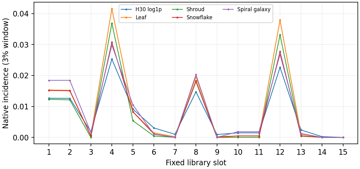
**Figure 2.** Fifteen-slot incidence profiles at $3\%$ tolerance. H30 uses its native transformed readout; the leaf, Shroud, snowflake and galaxy use their primary dark graphs. These are finite window-incidence profiles. The dark embryo results are reported in Table [1](/source-readout/cscf/09-spectral-evidence#tab-correlations).

<a id="section-10.3"></a>

### 10.3 Controls and robustness

Kerr’s development and angular-holdout 3% SUM incidences are $0.3058052$ and $0.3180936$. Table [2](/source-readout/cscf/09-spectral-evidence#tab-kerr) reports three conditional-reference comparisons. U conditions on observed endpoints and degeneracies while drawing transformed uniform groups. P retains labelled coarse raw-log bins and within-block circular phase differences, while shifting common within-bin phases. R preserves fitted overtone trends and within-$\ell$ residual Gram structure while rotating the two-dimensional residual complement. They preserve different, nonnested information. U and P discriminate in both datasets; R is more permissive on holdout.

<a id="tab-kerr"></a>

**Table 2.** Kerr conditional-reference comparisons \[[23](/source-readout/cscf/18-references#ref-spectral)\]. Each row uses 4,999 controls; $k$ counts scores at least the observation. The add-one fraction is $(k+1)/5000$, a summary under the stated reference law.

| Reference |  $B$ | $k_{\rm dev}$ | $k_{\rm hold}$ | $\Delta A_{\rm dev}$ | $\Delta A_{\rm hold}$ |
|:----------|-----:|--------------:|---------------:|---------------------:|----------------------:|
| U         | 4999 |             0 |              0 |              0.06041 |               0.07341 |
| P         | 4999 |            10 |             22 |              0.03901 |               0.05304 |
| R         | 4999 |            20 |            757 |              0.02518 |               0.00760 |

Hydrogen shell-block permutations retain the allowed support and each block’s full weight multiset while changing placement. The primary hydrogen–Kerr Spearman coefficient $0.521429$ has shell mean $0.521370$ and sample SD $0.002551$. Hydrogen–Shroud remains close to its observed $0.94868$ under the same reference. This establishes conditional profile robustness. Raw 3% UNION abundance is $0.1215927$ versus shell mean $0.1203374$, with no exceedance among 99 endpoints; transformed abundance is $0.1019029$ versus $0.1032113$, with 92 exceedances. The abundance response therefore depends on the readout. The short finite-fiber pilot moved too little to change the statistic and supplies no mixed-reference conclusion.

The original library’s three-domain paired reference fraction is $0.2339$, above the frozen $0.05$ criterion. The Kerr geometry-matched rank fractions were $0.0457$ in development and $0.0953$ on angular holdout. These library-specificity outcomes remain part of the evidence. They constrain a privilege claim for the chosen centers, while the measured recurrence and conditional-control results remain the phenomena represented by Theorem [9.1](/source-readout/cscf/08-modular-ratios#thm-modular).

<a id="section-10.4"></a>

### 10.4 Meaning within the common-carrier account

The spectral work establishes a recurring finite structural signature in specified constructions. The present paper establishes where that signature sits: it is a pooled spectral measure of $\Delta_\rho$ and a phase-difference readout of $\mathop{\mathrm{ad}}(\log V)$, both determined by the declared carrier and response. This supplies the proposed connection between visible organization and the coherent face with exact equations and the measured native profiles.

The representation holds for every admitted positive finite readout. It establishes the operator relationship independently of the recurrence’s empirical strength. The measured recurrence and its exact modular representation together support CSCF’s role as an organizing structure for source-to-readout spectral information. Selecting particular cross-domain profiles from physical realization laws is the next predictive development, addressed in Section [14](/source-readout/cscf/12-boundary-and-tests#sec-future).



## What closes after projection

Projection can lose information even when the source is exactly known. In a finite positive carrier the dissipative closure defect measures that loss, and regularity of the coherence symbol turns it into a bound on coherent leakage.

<a id="sec-probe"></a>

## 11. Observable quotients, memory and two-face closure

A field description must specify how it is accessed. Let $\mathcal X$ be a candidate state space, $\mathcal B$ a probe family and $R:\mathcal X\times\mathcal B\to\mathcal V$ its response map. Define

$$
x\sim_{\mathcal B}y\quad\Longleftrightarrow\quad R(x,b)=R(y,b)\ \text{for all }b\in\mathcal B.
$$

 The quotient retains exactly the distinctions available through those probes. Dissipative probes may sample $S_t$, $\Lambda_T$ or $\mathcal D_T$, while coherent probes may sample $U_s$, $\Gamma_T$ or $\mathfrak B_T$. Complete operator recovery, scalar-profile identifiability and finite window incidence have different information content. The factorization questions of Shadow Theory apply to each target with its declared probes \[[22](/source-readout/cscf/18-references#ref-sourcereadout), [20](/source-readout/cscf/18-references#ref-projecteddynamics)\].

<a id="section-11.1"></a>

### 11.1 Compression and exact projected dynamics

In finite dimension let $J:\mathbb C^k\to\mathsf H$ be an isometry, $P=JJ^*$ and $Q=I-P$. For a bounded linear generator $G$, the source equation $\dot y=Gy$ has resolved component $x=Py$ and unresolved component $z=Qy$. Solving the latter by variation of constants yields

<a id="eq-memory"></a>

$$
\begin{aligned}\dot x(t)={}&PGP x(t)+PGQ e^{tQGQ}z(0)\qquad\text{(12)}\\
&+\int_0^t PGQ e^{(t-s)QGQ}QGP x(s)\,ds.\end{aligned}
$$

The restricted exponentials act on $Q\mathsf H$. This identity retains the unresolved preparation and its dynamical return. It applies to the finite combined CSCF generator $G=-K-i h(K)$ as well as to $G=-K$. Dropping the last two terms requires an invariant-subspace or approximation argument. In the general quotient formulation, an induced evolution under a surjective linear readout $R$ exists precisely when its kernel is invariant under the source evolution \[[20](/source-readout/cscf/18-references#ref-projecteddynamics), Thm. 5.2\].

The response-kernel viewpoint also covers pairings such as $\mathop{\mathrm{Tr}}(\rho O)$, boundary input/output operators and scattering maps. Such a relational description is compatible with CSCF when its kernels are specified functions or compressions of $K$. A low-rank point-cloud approximation alone does not supply a physical carrier identification; its extraction and target must be independently specified. Here the empirical carriers are the actual finite operators declared in Section [10](/source-readout/cscf/09-spectral-evidence#sec-empirical).

<a id="section-11.2"></a>

### 11.2 An exact dissipative closure certificate

Set

<a id="eq-defect"></a>

$$
A(t)=J^*e^{-tK}J,\qquad B(t)=Qe^{-tK}J,\qquad
M(t)=A(2t)-A(t)^2.\tag{13}
$$

<a id="thm-gram"></a>

**Theorem 11.1.** *Gram defect and closure*.

For finite selfadjoint $K\ge0$ and all $t,s\ge0$,

$$
A(t+s)-A(t)A(s)=B(t)^*B(s),\qquad M(t)=B(t)^*B(t)\ge0.
$$

 At any fixed $\tau>0$, $M(\tau)=0$ if and only if $[P,K]=0$. In that case the compressed dissipative evolution closes exactly, and the same subspace reduces $h(K)$ and every coherent flow $U_s$.

*Proof.* Insert $I=P+Q$ between the commuting selfadjoint operators $e^{-tK}$ and $e^{-sK}$. The $P$ term gives $A(t)A(s)$ and the $Q$ term gives $B(t)^*B(s)$. If $M(\tau)=0$, then $B(\tau)=0$, so $P\mathsf H$ is invariant under $e^{-\tau K}$. Selfadjointness also makes its orthogonal complement invariant. Therefore $P$ commutes with that operator and with $K=-\tau^{-1}\log(e^{-\tau K})$. The converse follows directly. Functional calculus then implies $[P,h(K)]=[P,U_s]=0$. ◻

For reversible finite-state Markov dynamics this is the equilibrium-weighted certificate of the effective-autonomy study \[[1](/source-readout/cscf/18-references#ref-roundfour), Sec. 6\]. Weighting is part of the correspondence: for row generator $Q_{\rm M}$, strictly positive stationary law $\pi$ and partition incidence matrix $C_{\rm part}$ with nonempty blocks,

$$
K=-D_\pi^{1/2}Q_{\rm M}D_\pi^{-1/2},\qquad
J=D_\pi^{1/2}C_{\rm part}D_{\bar\pi}^{-1/2},\quad \bar\pi=\pi C_{\rm part}.
$$

 Here $\pi$ is written as a row vector in $\bar\pi=\pi C_{\rm part}$, and $D_\pi$ and $D_{\bar\pi}$ are diagonal probability matrices. Then $J^*J=I$. Unweighted matrices for a nonuniform equilibrium generally do not satisfy the symmetric formula. The coherent invariance statement concerns a Hilbert subspace; its reduced unitary is not thereby a stochastic transition matrix.

<a id="section-11.3"></a>

### 11.3 Quantitative transfer to the coherent face

<a id="thm-closure-coherence"></a>

**Theorem 11.2.** *Closure-to-coherence transfer*.

Suppose $0\le K\le\Lambda I$ in finite dimension, and let $h$ be real and Lipschitz on $\mathop{\mathrm{\sigma}}K$, with constant $L_h$. For $\tau>0$ and $t\in\mathbb R$,

<a id="eq-transfer"></a>

$$
\left\lVert Qe^{-it h(K)}J\right\rVert_F\le
\min\left\{\sqrt{k},\ \frac{|t|L_h e^{\Lambda\tau}}{\tau}
\sqrt{\mathop{\mathrm{Tr}}M(\tau)}\right\}.\tag{14}
$$

Here $\left\lVert\cdot\right\rVert_F$ denotes the Frobenius norm. In particular,

<a id="eq-generator-transfer"></a>

$$
\left\lVert Qh(K)J\right\rVert_F\le L_h\left\lVert QKJ\right\rVert_F,
\quad
\tau e^{-\Lambda\tau}\left\lVert QKJ\right\rVert_F
\le\sqrt{\mathop{\mathrm{Tr}}M(\tau)}\le\tau\left\lVert QKJ\right\rVert_F.\tag{15}
$$

*Proof.* In an orthonormal eigenbasis of $K$, the entries of $[P,f(K)]$ are $P_{ij}(f(\lambda_j)-f(\lambda_i))$. For Hermitian $F$, its two off-diagonal blocks relative to $P$ have equal Frobenius norm, giving

$$
\left\lVert[P,F]\right\rVert_F^2=2\left\lVert QFJ\right\rVert_F^2.
$$

 The same equality holds for $F=e^{-it h(K)}$: it is normal and diagonal in this eigenbasis, or directly its two block norms agree by unitarity. The scalar bounds

$$
\begin{aligned}
|h(\lambda)-h(\mu)|&\le L_h|\lambda-\mu|,\\
|e^{-it h(\lambda)}-e^{-it h(\mu)}|&\le |t|L_h|\lambda-\mu|,\\
\tau e^{-\Lambda\tau}|\lambda-\mu|
&\le |e^{-\tau\lambda}-e^{-\tau\mu}|
\le\tau|\lambda-\mu|
\end{aligned}
$$

 follow from Lipschitz continuity, the unit-circle chord estimate and the mean-value theorem. Summing squared commutator entries proves [(15)](/source-readout/cscf/10-quotient-closure#eq-generator-transfer) and bounds the unitary leakage by $|t|L_h\left\lVert QKJ\right\rVert_F$. Theorem [11.1](/source-readout/cscf/10-quotient-closure#thm-gram) identifies $\left\lVert Qe^{-\tau K}J\right\rVert_F^2$ with $\mathop{\mathrm{Tr}}M(\tau)$. Finally unitarity and $J^*J=I$ give the ceiling $\sqrt{k}$. ◻

The proof uses a Hilbert–Schmidt estimate, not an operator-Lipschitz claim for arbitrary functions. For $h(\lambda)=(2/\pi)\arctan(\lambda/\lambda_0)$, one may take $L_h=2/(\pi\lambda_0)$. The factor $e^{\Lambda\tau}$ explains why late-time near-stationarity can yield a weak inverse estimate. A useful measurement therefore declares bandwidth and lag as well as the symbol.

If an estimated Hermitian defect $\widehat M$ obeys $\left\lVert\widehat M-M\right\rVert_{\rm op}\le\delta$, then $\mathop{\mathrm{Tr}}M\le\mathop{\mathrm{Tr}}\widehat M+k\delta$. Thus replacing the square root in [(14)](/source-readout/cscf/10-quotient-closure#eq-transfer) by $\sqrt{\max\{0,\mathop{\mathrm{Tr}}\widehat M+k\delta\}}$ gives a valid conservative bound whenever the stated error certificate holds. This separates measurement precision from an exact closure identity.



## Physical realizations and reciprocal memory

A rate law requires more than curvature. Mobility, internal storage and the physical response contract determine which carrier the observer measures.

<a id="sec-physical-realizations"></a>

## 12. Physical realizations, reciprocal memory and response

The common-carrier construction has concrete realizations in relaxation theory, reversible stochastic dynamics and aligned complex-amplitude dynamics. A physical realization specifies both the curvature functional and the metric that converts a functional derivative into a rate. It also specifies a coherence law and a probe space. These data determine which parts of the abstract spectral calculus represent measured rates, physical frequencies and observable transfer functions.

<a id="section-12.1"></a>

### 12.1 Mobility converts curvature into a relaxation carrier

Let $q\in\mathbb R^N$ be local coordinates, let $F\in C^2$ be an energy or dimensionless thermodynamic potential, and consider

<a id="eq-physical-gradient"></a>

$$
\dot q=-M(q)\nabla F(q),\qquad M(q)=M(q)^\top>0.\tag{16}
$$

The coordinates and mobility include the physical unit conversions. For example, if $F$ has energy units, the entries of $M$ convert its coordinate gradient into coordinate velocity. Throughout this subsection the metric is finite dimensional and nonsingular. Entropy-gradient constructions and detailed-balance geometries provide important physical instances of this choice \[[6](/source-readout/cscf/18-references#ref-carlenmaas)\].

<a id="lem-mobility-whitened"></a>

**Lemma 12.1.** *Mobility-whitened curvature*.

Suppose $q_*$ is a stationary point of $F$, $M$ is continuous at $q_*$, and $H=\mathop{\mathrm{Hess}}F(q_*)$ is positive semidefinite. Set $M_*=M(q_*)$ and $y=M_*^{-1/2}(q-q_*)$. The linearization of [(16)](/source-readout/cscf/11-physical-realizations#eq-physical-gradient) is

<a id="eq-mobility-carrier"></a>

$$
\dot y=-K_*y,\qquad K_*=M_*^{1/2}HM_*^{1/2}\geq0.\tag{17}
$$

Thus $K_*$ is selfadjoint in the whitened Euclidean Hilbert space, and its eigenvalues have units of inverse time. If $H>0$, all linearized modes decay strictly.

*Proof.* At a stationary point $\nabla F(q_*)=0$. Continuity gives $M(q_*+\delta q)=M_*+o(1)$, while $\nabla F(q_*+\delta q)=H\delta q+o(|\delta q|)$. Their product is $M_*H\delta q+o(|\delta q|)$, so $\delta\dot q=-M_*H\delta q$. Substitution of $\delta q=M_*^{1/2}y$ gives [(17)](/source-readout/cscf/11-physical-realizations#eq-mobility-carrier). Symmetry and positivity follow from $y^\top K_*y=(M_*^{1/2}y)^\top H(M_*^{1/2}y)$. The matrices $M_*H$ and $K_*$ are similar, so this change of representation preserves the complete relaxation spectrum and its multiplicities. ◻

The Hessian and the physical generator therefore coincide only after the metric has been specified. For a state-dependent mobility the lemma remains a local result at a stationary state; it does not freeze the mobility along an arbitrary nonlinear trajectory. If zero modes occur, the positive spectral subspace and any conserved coordinates must be identified before forming inverse-rate observables.

<a id="section-12.2"></a>

### 12.2 Reciprocal storage, the full Hessian and exact memory

Consider a reciprocal-storage model \[[3](/source-readout/cscf/18-references#ref-roundtwo), Sec. 4\] with visible coordinates $x\in\mathbb R^n$ and internal coordinates $m\in\mathbb R^k$. To distinguish storage stiffness from the CSCF carrier, write its potential as

<a id="eq-reciprocal-potential"></a>

$$
F(x,m)=V_0(x)+\frac12m^\top Rm-m^\top r(x),\qquad R=R^\top>0,\tag{18}
$$

where $V_0$ and $r$ are $C^2$ and all terms have the same potential units. Choose time and coordinate scales so that the mobilities are $I_n$ and $\epsilon I_k$, with $\epsilon>0$. The full deterministic dynamics is

<a id="eq-reciprocal-dynamics"></a>

$$
\dot x=-\nabla_xF(x,m),\qquad
 \dot m=-\epsilon\nabla_mF(x,m)
       =\epsilon\{r(x)-Rm\}.\tag{19}
$$

Both directions of the interaction derive from the same potential. Its dissipation law is exact:

<a id="eq-reciprocal-dissipation"></a>

$$
\frac{dF}{dt}=-|\nabla_xF|^2-\epsilon|\nabla_mF|^2\leq0.\tag{20}
$$

<a id="prop-storage-hessian"></a>

**Proposition 12.2.** *Static reduction and the physical carrier*.

Define

<a id="eq-storage-effective-potential"></a>

$$
F_{\mathrm{eff}}(x)=V_0(x)-\frac12r(x)^\top R^{-1}r(x).\tag{21}
$$

Joint stationary points are precisely $(x_*,m_*)=(x_*,R^{-1}r(x_*))$, with $\nabla F_{\mathrm{eff}}(x_*)=0$. At such a point, write

<a id="eq-storage-full-hessian"></a>

$$
H=\mathop{\mathrm{Hess}}F(x_*,m_*)=
 \begin{pmatrix}A&-C\\-C^\top&R\end{pmatrix},\qquad
 C=Dr(x_*)^\top.\tag{22}
$$

Then

<a id="eq-storage-schur"></a>

$$
S=A-CR^{-1}C^\top=\mathop{\mathrm{Hess}}F_{\mathrm{eff}}(x_*),\qquad
 H>0\ \Longleftrightarrow\ S>0.\tag{23}
$$

At a nondegenerate strict minimum the complete linearized relaxation carrier is

<a id="eq-storage-full-carrier"></a>

$$
K_*=M^{1/2}HM^{1/2},\qquad
 M=\operatorname{diag}(I_n,\epsilon I_k).\tag{24}
$$

This conclusion holds for every $\epsilon>0$.

*Proof.* Completion of the square gives the identity

<a id="eq-storage-square"></a>

$$
F(x,m)=F_{\mathrm{eff}}(x)+
 \frac12\{m-R^{-1}r(x)\}^\top R\{m-R^{-1}r(x)\}.\tag{25}
$$

The stationary-point statement follows by differentiation. For vectors $u\in\mathbb R^n$ and $v\in\mathbb R^k$,

<a id="equation-26"></a>

$$
\begin{pmatrix}u\\v\end{pmatrix}^{\!\top}
 H\begin{pmatrix}u\\v\end{pmatrix}
 =u^\top Su+(v-R^{-1}C^\top u)^\top R(v-R^{-1}C^\top u).\tag{26}
$$

This proves the Schur-complement criterion and identifies the reduced Hessian. Lemma [12.1](/source-readout/cscf/11-physical-realizations#lem-mobility-whitened) gives the complete carrier. ◻

The same model gives a memory representation without an adiabatic approximation:

<a id="eq-exact-storage-memory"></a>

$$
m(t)=e^{-\epsilon Rt}m(0)+
       \epsilon\int_0^t e^{-\epsilon R(t-u)}r(x(u))\,du.\tag{27}
$$

Thus internal retention, static feedback and transient response are three representations of the same reciprocal interaction. The initial-condition term in [(27)](/source-readout/cscf/11-physical-realizations#eq-exact-storage-memory) remains part of the transient law.

For a small force $f$ added to the $x$ equation at a stationary point, let $p$ denote the Laplace frequency, with units of inverse time. For zero perturbation initial conditions,

<a id="equation-28"></a>

<a id="equation-29"></a>

$$
\begin{aligned}p\delta x&=-A\delta x+C\delta m+f,\qquad\text{(28)}\\
p\delta m&=\epsilon C^\top\delta x-\epsilon R\delta m.\qquad\text{(29)}\end{aligned}
$$

Eliminating the internal perturbation gives the inverse susceptibility

<a id="eq-storage-susceptibility"></a>

$$
\chi_{xx}(p)^{-1}=pI+A-
 \epsilon C(pI+\epsilon R)^{-1}C^\top.\tag{30}
$$

Its static limit is $S$, whereas the internal correction vanishes at large $|p|$ away from poles. The static Schur complement describes relaxed curvature. The $(n+k)$-dimensional carrier in [(24)](/source-readout/cscf/11-physical-realizations#eq-storage-full-carrier) retains the internal relaxation modes needed for the full response. This distinction prevents static elimination from changing the transient physical problem.

<a id="section-12.3"></a>

### 12.3 A positive carrier with hidden cross-response

Consider the dimensionless reciprocal-storage potential \[[2](/source-readout/cscf/18-references#ref-roundthree), Sec. 9\],

<a id="eq-three-coordinate-potential"></a>

$$
F(a,b,z)=\frac14(a^2-1)^2+\frac14(b^2-1)^2+
          \frac12(z-ab)^2.\tag{31}
$$

Use unit mobility and the chosen dimensionless time unit. At the minimum $(a,b,z)=(1,1,1)$ the complete Hessian is

<a id="eq-three-coordinate-h"></a>

$$
K=H=\begin{pmatrix}3&1&-1\\1&3&-1\\-1&-1&1\end{pmatrix}.\tag{32}
$$

Its leading principal minors are $3,8,4$, and

<a id="equation-33"></a>

$$
\mathop{\mathrm{\sigma}}(K)=\left\{2,\frac{5-\sqrt{17}}2,
                        \frac{5+\sqrt{17}}2\right\}>0.\tag{33}
$$

Consequently $e^{-tK}$ is the exact linearized relaxation semigroup. For a force in the $a$ coordinate and observation in the $b$ coordinate, the transfer function is

<a id="eq-hidden-cross-response"></a>

$$
\chi_{ba}(p)=e_b^\top(pI+K)^{-1}e_a
 =-\frac{p}{(p+2)(p^2+5p+2)}.\tag{34}
$$

To verify this expression, the antisymmetric coordinate $(a-b)/\sqrt2$ has rate $2$, while the symmetric coordinate and $z$ have the $2\times2$ block $\left(\begin{smallmatrix}4&-\sqrt2\\-\sqrt2&1\end{smallmatrix}\right)$. Hence

<a id="equation-35"></a>

$$
\chi_{ba}(p)=\frac12\left\{
 \frac{p+1}{p^2+5p+2}-\frac1{p+2}\right\},\tag{35}
$$

which reduces to [(34)](/source-readout/cscf/11-physical-realizations#eq-hidden-cross-response). The static cross-response vanishes, $\chi_{ba}(0)=0$, although the frequency-dependent cross-response is nonzero. The three poles are not cancelled by the numerator. This example makes the role of observable projection explicit: the carrier, its mode multiplicities and the probe vectors jointly determine the measured response. An eigenvalue distribution alone does not specify those probe overlaps. Once a coherence symbol is declared, the same $K$ also supplies $h(K)$ and its unitary flow; the response calculation fixes $K$, not a unique physical coherence law.

<a id="section-12.4"></a>

### 12.4 Detailed balance and stochastic-matrix-form carriers

Let $Q$ be the row generator of a finite continuous-time Markov chain, so $Q_{ij}\geq0$ for $i\ne j$, $Q\mathbf1=0$, and the rates have units of inverse time. Suppose its strictly positive stationary distribution $\pi$ satisfies detailed balance $\pi_iQ_{ij}=\pi_jQ_{ji}$. For $D=\operatorname{diag}(\pi)$ define

<a id="eq-rk-carrier"></a>

$$
K=-D^{1/2}QD^{-1/2}.\tag{36}
$$

This is the finite-dimensional stochastic-matrix-form correspondence \[[7](/source-readout/cscf/18-references#ref-rk)\]. Detailed balance makes $K$ real symmetric, and for $u=D^{1/2}f$,

<a id="eq-rk-dirichlet"></a>

$$
u^\top Ku=\frac12\sum_{i,j}\pi_iQ_{ij}(f_i-f_j)^2\geq0.\tag{37}
$$

Moreover,

<a id="equation-38"></a>

$$
e^{-tK}=D^{1/2}e^{tQ}D^{-1/2},\qquad K\sqrt\pi=0.\tag{38}
$$

The similarity preserves rates and multiplicities exactly. The stationary vector is retained as a zero mode, or removed by an explicit restriction to its orthogonal complement when required.

For example, take

<a id="equation-39"></a>

$$
\pi=\frac1{14}(1,4,9)^\top,\quad
 Q=\begin{pmatrix}-3&2&1\\1/2&-5/4&3/4\\1/9&1/3&-4/9\end{pmatrix}.\tag{39}
$$

Then

<a id="equation-40"></a>

$$
K=\begin{pmatrix}3&-1&-1/3\\-1&5/4&-1/2\\-1/3&-1/2&4/9\end{pmatrix},
 \qquad K(1,2,3)^\top=0.\tag{40}
$$

Its off-diagonal conductances are $\pi_iQ_{ij}$, so the equilibrium weight is an essential part of the representation. An associated quantum Hamiltonian may be defined as $\hbar\alpha K$, with dimensionless conversion factor $\alpha$; its unitary evolution is $e^{-i\alpha tK}$. This construction identifies corresponding spectra after the stated unit conversion. For a finite spectral cutoff, the symbol $h(\lambda)=\alpha\lambda$ on the retained interval can be extended constantly above that interval, giving a bounded nondecreasing symbol when $\alpha\geq0$.

<a id="section-12.5"></a>

### 12.5 An aligned complex-gradient realization

The variational complex Ginzburg–Landau equation on its parameter line $b=c$ has, after a rotating-frame change, dissipative and reactive terms generated by one real functional \[[4](/source-readout/cscf/18-references#ref-aranson), Sec. II.A\]. The pertinent finite-dimensional structure can be stated without a continuum-domain ambiguity. Let $\mathcal J$ be an orthogonal complex structure on $\mathbb R^{2N}$, so $\mathcal J^\top=-\mathcal J$ and $\mathcal J^2=-I$, and set

<a id="eq-aligned-gradient"></a>

$$
\dot q=-(\gamma I+\alpha\mathcal J)\nabla F(q),\qquad\gamma>0.\tag{41}
$$

The coefficients include any factor from the convention for the Wirtinger derivative $\delta F/\delta z^*$. The exact balance is $dF/dt=-\gamma|\nabla F|^2$.

<a id="prop-complex-alignment"></a>

**Proposition 12.3.** *A sufficient same-carrier alignment condition*.

At a stationary state let $H=\mathop{\mathrm{Hess}}F\geq0$ and assume $[H,\mathcal J]=0$. Identify $\mathcal J$ with multiplication by $i$ on $\mathbb C^N$. Then $H$ represents a complex Hermitian operator $K\geq0$, and the linearized evolution of [(41)](/source-readout/cscf/11-physical-realizations#eq-aligned-gradient) is

<a id="eq-complex-aligned-factorization"></a>

$$
z(t)=e^{-\gamma tK}e^{-i\alpha tK}z(0).\tag{42}
$$

The relaxation rates and phase frequencies are respectively $\gamma\lambda_j$ and $\alpha\lambda_j$ on the same eigenspaces.

*Proof.* Commutation with $\mathcal J$ makes $H$ complex linear. Its real symmetry then gives complex Hermitian symmetry, and real positivity gives $K\geq0$. The linearized generator is $-(\gamma+i\alpha)K$. Its real and imaginary parts commute, proving [(42)](/source-readout/cscf/11-physical-realizations#eq-complex-aligned-factorization); also $d|z|^2/dt=-2\gamma\langle z,Kz\rangle$. ◻

For example, on a finite graph take $K=\mu I+\kappa L$ with $\mu>0$, $\kappa\geq0$ and $L$ a positive graph Laplacian. The quadratic energy $F(q)=q^\top Hq/2$ with this complex-linear $H$ has the required alignment. A quartic complex-amplitude energy has the same linearization at zero when its quadratic part is this $K$. At a general nonzero amplitude its real Hessian can couple $\delta z$ to $\delta\bar z$; the alignment must then be checked at that state. With dissipative carrier $K_d=\gamma K$, the physical coherence symbol on its finite spectrum is $h(\lambda)=(\alpha/\gamma)\lambda$. A bounded monotone extension is available for $\alpha\geq0$. For a continuum model one must additionally specify boundary conditions, the closed energy form, the operator domain and the retained cutoff; the finite-dimensional proposition does not supply those data.

<a id="section-12.6"></a>

### 12.6 Quantum and experimental response anchors

Quantum detailed-balance generators provide a related operator-space realization \[[9](/source-readout/cscf/18-references#ref-firanko)\]. For a declared detailed-balance inner product $\langle X,Y\rangle_W=\langle X,WY\rangle_{\mathrm{HS}}$, where $W>0$ is the metric superoperator, a nonpositive selfadjoint Heisenberg generator $\mathcal L$ becomes $\mathcal K=-W^{1/2}\mathcal L W^{-1/2}\geq0$ in Hilbert–Schmidt coordinates. The stationary state, the convention for detailed balance and the chosen picture determine $W$. The cited local Hamiltonian construction supplies stronger locality conclusions under its additional term hypotheses. The corresponding Hamiltonian is the Hermitian representative of the relaxation generator; its identification with another independently specified physical Hamiltonian is an additional model equation.

Fluctuation–response relations and projection methods \[[12](/source-readout/cscf/18-references#ref-kubo), [13](/source-readout/cscf/18-references#ref-mori)\] connect measured susceptibility, equilibrium correlations and memory kernels. Equation [(30)](/source-readout/cscf/11-physical-realizations#eq-storage-susceptibility) is an explicit finite model in this response programme. It preserves the internal poles instead of replacing them by a static effective stiffness. In an experiment, probe vectors, temperature, preparation and the frequency convention accompany the spectral carrier.

Optical temporal coupled-mode theory offers a direct test platform \[[26](/source-readout/cscf/18-references#ref-suh)\]. With the convention $a(t)\sim e^{-i\omega t}$, write

<a id="equation-43"></a>

$$
\dot a=(-i\Omega-\Gamma)a+B s_{\mathrm{in}},\qquad
 \Omega=\Omega^*,\quad\Gamma=\Gamma^*\geq0.\tag{43}
$$

The opposite phasor convention reverses the sign of the frequency term. For amplitudes normalized so that $|a|^2$ is stored energy, passive port loss obeys $D^*D=2\Gamma$ when all decay is assigned to those ports. Here $\Gamma$ has units of inverse time and $\Omega$ of angular frequency. An exact CSCF realization requires a nominated law $\Omega=h(\Gamma)$ after any declared carrier-frequency subtraction. In particular $[\Omega,\Gamma]=0$, and $\Omega$ must be scalar on every degenerate eigenspace of $\Gamma$. Commutation alone does not impose that scalar-on-block condition. The joint measurement of decay, frequency and modal overlaps can therefore test the same-carrier law more sharply than two unrelated spectral fits. General reversible–irreversible frameworks \[[10](/source-readout/cscf/18-references#ref-generic)\] provide broader physical context; the aligned common-carrier realization is a specified subclass within that larger setting.



## Boundary carriers and discriminating tests

A boundary carrier gives a concrete place to test the two faces together. The same geometry must supply the form, mobility, time scale and retained observables before a response comparison becomes a physical test.

<a id="sec-realization"></a>

## 13. Boundary realization and physical discrimination

The form construction can also arise after a boundary reduction. The correct object is then the boundary energy induced by a specified bulk problem, including its boundary conditions and boundary Hilbert metric. A positive bulk differential expression alone does not select that energy or its Dirichlet-to-Neumann operator.

<a id="section-13.1"></a>

### 13.1 An explicit curvature-to-boundary carrier

The following finite-mode collar construction supplies an exact example. Let $H_b=\mathbb C^N$, let $B\geq0$ be Hermitian with eigenvalues $m_j$, and let $\beta>0$. For $u\in H^1([0,\beta];H_b)$ consider the bulk energy

$$
\mathcal E(u)=\int_0^\beta\big(\left\lVert u'(x)\right\rVert^2+\left\lVert Bu(x)\right\rVert^2\big)\,dx.
$$

 Fix $u(0)=f$ and leave the other boundary free. The resulting natural condition is $u'(\beta)=0$.

<a id="prop-collar"></a>

**Proposition 13.1.** *Collar boundary carrier*.

The minimum boundary energy is the closed nonnegative form

$$
Q_\partial(f)=\min_{u(0)=f}\mathcal E(u)
=\langle f,K_\partial f\rangle,\qquad
K_\partial=B\tanh(\beta B).
$$

 In the $j$th mode its unique minimizing extension and outward derivative are

$$
u_j(x)=f_j\frac{\cosh[m_j(\beta-x)]}{\cosh(m_j\beta)},\qquad
-u_j'(0)=m_j\tanh(m_j\beta)f_j.
$$

 At $m_j=0$ the extension is constant and the boundary rate is zero.

*Proof.* Modewise variation gives $-u_j''+m_j^2u_j=0$ with the stated mixed boundary data, solved by the displayed formula. Its energy is

$$
\int_0^\beta(|u_j'|^2+m_j^2|u_j|^2)\,dx
=[\overline{u_j}u_j']_0^\beta
=m_j\tanh(m_j\beta)|f_j|^2.
$$

 The integration by parts uses the mode equation and the zero derivative at $\beta$. If $v$ has $v(0)=0$, the cross term between the solution and $v$ vanishes by the same identity; hence $\mathcal E(u+v)=\mathcal E(u)+\mathcal E(v)$. The latter is strictly positive for nonzero such $v$, including the zero-mass sector. This proves minimality and uniqueness. Summing modes gives $K_\partial$ and its nonnegative form. ◻

The construction preserves the boundary amplitudes, their multiplicities and the bulk boundary conditions. Replacing the free endpoint by another condition would define another carrier. A physical boundary mobility converts this curvature to rates as in Lemma [12.1](/source-readout/cscf/11-physical-realizations#lem-mobility-whitened). An independently specified $h$ then yields the coherent face of that same boundary carrier. In an infinite-dimensional extension, trace spaces, closedness and operator domains must be supplied; finite retained-mode budgets already obey the results proved here.

<a id="section-13.2"></a>

### 13.2 What a joint physical test measures

A paired physical realization supplies more information than separate lists of decay rates and frequencies. It specifies an isometry or metric conversion, a retained subspace, physical time and a law $C=h(K)$ in those coordinates. With preparation $b$ and observation $a$, its dissipative transfer is $\langle a,(p+K)^{-1}b\rangle$, while the nominated coherent response is $\langle a,e^{-it h(K)}b\rangle$. These contain probe overlaps as well as eigenvalues. Optical mode measurements can test the common eigenspaces and the scalar-on-degenerate-block condition directly. Projected measurements can test $M(\tau)$ and the bandwidth-dependent bound of Theorem [11.2](/source-readout/cscf/10-quotient-closure#thm-closure-coherence).

This provides three connected levels of evidence. Native spectral profiles describe measured organization in a declared carrier. Operator identities locate those profiles in its coherent and modular calculus. Joint physical response measurements test a specified realization of the paired faces. Keeping these levels explicit allows the mathematical results to be used firmly at their actual strength.

<a id="sec-future"></a>

## 14. Future work: selection of profiles by physical realization laws

The next theoretical task is to derive particular recurring profiles from physical realization laws. Such a result would begin with an admitted source branch, its functional, metric, boundary data and preparation, and predict the resulting $K$, native $g$ and spectral-window profile before comparison. The present paper establishes the operator location of the profile and its response architecture. The selection problem asks why the resulting measure has one distribution rather than another.

Several tractable developments follow from this foundation. First, paired-response systems can nominate $h$ from physical units and a constitutive law, then compare frequency and attenuation responses in a common modal basis. Second, retained internal variables produce families of local curvature carriers through the full potential and mobility. A nonautonomous $K(t)$ need not commute with $K(s)$, so extending the fixed-carrier theory requires an evolution-family construction rather than substitution into a constant-generator exponential. Third, boundary and continuum realizations can extend the finite budgets only after a determinant convention and its renormalization laws have been fixed. Finally, new spectral measurements can test profile predictions with frozen readouts, structured controls and independently acquired data. These are subsequent physical and predictive developments of the architecture derived here.

<a id="section-15"></a>

## 15. Conclusion

CSCF combines the historical Lambda and coherence constructions into one spectral field. A closed curvature form and Hilbert metric determine $K$; a declared coherence symbol determines its reversible face, while the same carrier supplies contraction, averaged transmission and spectral budgets. Exact transmission recovery, profile identifiability and observable closure make this architecture accessible through defined readouts.

The recurring structures of the completed spectral investigation now have an explicit mathematical place in that account. Their ordered ratios are the modular spectrum of the retained positive readout, and their log differences are a coherent commutator spectrum. The exact connection preserves the native measurements and all their recorded heterogeneity. The closure-to-coherence theorem further transfers a quantitative observable constraint between the two faces. Worked relaxation, storage, detailed-balance, complex-gradient and boundary realizations show how the same architecture enters physical response. Within Shadow Theory, this is the field layer through which an admitted spectral realization is organized into coherent and dissipative readouts. Deriving the particular cross-domain profiles from physical realization laws is the next stage of the programme.



## Appendix A: Functional calculus details

<a id="app-fc"></a>

## A. Functional Calculus Details

##### A.1 Borel functional calculus.

For $K$ selfadjoint with $E_K$, the map $\phi \mapsto \phi(K) = \int \phi\, dE_K$ is a $*$-homomorphism from bounded Borel functions on $\mathop{\mathrm{\sigma}}(K)$ into $B(\mathsf H)$, with $\|\phi(K)\| = \|\phi\|_{L^\infty(E_K)}$. Unbounded Borel $\phi$ gives densely defined $\phi(K)$, selfadjoint when $\phi$ is real.

##### A.2 Stone’s theorem.

Every strongly continuous one-parameter unitary group $(U_t)$ on $\mathsf H$ has a unique selfadjoint generator $\widetilde C$ with $U_t = e^{-it\widetilde C}$. Boundedness of $\widetilde C$ is equivalent to operator-norm continuity of $(U_t)$.



## Appendix B: When the Lambda profile is injective

<a id="app-profile-inj"></a>

## B. Lambda-Profile Injectivity on Compact Positive Supports

<a id="thm-lambda-profile-injectivity"></a>

**Theorem B.1.** *Lambda-profile injectivity*.

Let $\mu$ be a finite positive Borel measure supported on a compact interval $[a,b]\subset(0,\infty)$, and define

$$
F_\mu(T) \;=\; \int_{[a,b]} -\log(1-e^{-T\lambda})\,d\mu(\lambda),\qquad T>0.
$$

 If $\mu_1,\mu_2$ are finite positive Borel measures supported in $[a,b]$ and $F_{\mu_1}(T) = F_{\mu_2}(T)$ for all $T>0$, then $\mu_1 = \mu_2$.

*Proof.* Write $\phi(x) := -\log(1-e^{-x})$ for $x>0$. We first establish a Mellin representation, then deduce $\mu_1 = \mu_2$ from equality of moments after a change of variable.

*Step 1: Mellin representation.* For $\Re s = \sigma > 0$ we show

$$
\int_0^\infty T^{s-1} F_\mu(T)\,dT \;=\; \Gamma(s)\,\zeta(s+1)\int_{[a,b]}\lambda^{-s}\,d\mu(\lambda).
$$

 For $0<T\le 1$ and $\lambda\in[a,b]$,

$$
1 - e^{-T\lambda} \;=\; T\lambda\int_0^1 e^{-\theta T\lambda}\,d\theta \;\ge\; T a\, e^{-b},
$$

 so

$$
\phi(T\lambda) \;\le\; b - \log a - \log T,
$$

 which is integrable against $T^{\sigma-1}$ at $T=0$. For $T\ge 1$,

$$
\phi(T\lambda) \;=\; -\log(1-e^{-T\lambda}) \;\le\; \frac{e^{-T\lambda}}{1-e^{-T\lambda}} \;\le\; \frac{e^{-aT}}{1-e^{-a}},
$$

 which is integrable against $T^{\sigma-1}$ at $T=\infty$. Since $\mu$ is finite, the same bounds justify integrating against $d\mu(\lambda)$.

For fixed $\lambda>0$,

$$
-\log(1-e^{-T\lambda}) \;=\; \sum_{n\ge 1}\frac{e^{-nT\lambda}}{n}.
$$

 For $\sigma>0$,

$$
\sum_{n\ge 1}\frac{1}{n}\int_0^\infty T^{\sigma-1} e^{-nT\lambda}\,dT \;=\; \Gamma(\sigma)\,\lambda^{-\sigma}\sum_{n\ge 1} n^{-(\sigma+1)} \;<\;\infty,
$$

 so termwise integration is justified and

$$
\int_0^\infty T^{s-1}\big[-\log(1-e^{-T\lambda})\big]\,dT \;=\; \Gamma(s)\,\zeta(s+1)\,\lambda^{-s},\qquad \Re s>0.
$$

 Since $\int_{[a,b]} \lambda^{-\sigma}\,d\mu(\lambda) < \infty$ on the compact interval $[a,b]\subset(0,\infty)$, Fubini–Tonelli applies, yielding the displayed identity.

*Step 2: From profile equality to moment equality.* Assume $F_{\mu_1}(T) = F_{\mu_2}(T)$ for all $T>0$. Taking the Mellin transform on $\Re s>0$ (real $s>0$ suffices),

$$
\Gamma(s)\,\zeta(s+1)\int_{[a,b]} \lambda^{-s}\,d\mu_1(\lambda) \;=\; \Gamma(s)\,\zeta(s+1)\int_{[a,b]} \lambda^{-s}\,d\mu_2(\lambda).
$$

 For real $s>0$, $\Gamma(s)>0$ and $\zeta(s+1)>1$, so

$$
\int_{[a,b]} \lambda^{-s}\,d\mu_1(\lambda) \;=\; \int_{[a,b]} \lambda^{-s}\,d\mu_2(\lambda),\qquad s>0.
$$

*Step 3: Recovery of total mass and Weierstrass closure.* Let $\eta_i$ be the pushforward of $\mu_i$ under the homeomorphism

$$
[a,b] \to [1/b,1/a],\qquad \lambda \mapsto x = \lambda^{-1}.
$$

 Then

$$
\int_{[1/b,1/a]} x^s\,d\eta_1(x) \;=\; \int_{[1/b,1/a]} x^s\,d\eta_2(x),\qquad s>0.
$$

 Taking $s\downarrow 0$, $x^s \to 1$ uniformly on $[1/b,1/a]$, so the total masses agree:

$$
\eta_1([1/b,1/a]) \;=\; \eta_2([1/b,1/a]).
$$

 For $s = n \in \mathbb N$ this gives equality of all positive integer moments. Combined with the zeroth moment, all polynomial moments agree:

$$
\int p(x)\,d\eta_1(x) \;=\; \int p(x)\,d\eta_2(x) \qquad \text{for every polynomial } p.
$$

 By Weierstrass approximation, polynomials are uniformly dense in $C([1/b,1/a])$, so

$$
\int f(x)\,d\eta_1(x) \;=\; \int f(x)\,d\eta_2(x)\qquad \text{for every } f\in C([1/b,1/a]).
$$

 By the uniqueness clause of the Riesz representation theorem, $\eta_1 = \eta_2$. Pulling back along the homeomorphism $\lambda \mapsto 1/\lambda$ yields $\mu_1 = \mu_2$. ◻

<a id="cor-finite-rank-profile"></a>

**Corollary B.2.** *Finite-rank spectra*.

Let $K_1, K_2$ have finite positive spectra contained in $[a,b]\subset(0,\infty)$.

1.  If the unnormalized counting measures $\nu_{K_i} = \sum_{\lambda\in\mathop{\mathrm{\sigma}}(K_i)\cap(0,\infty)} m_i(\lambda)\,\delta_\lambda$ have equal Lambda profiles $F_{\nu_{K_1}}(T) = F_{\nu_{K_2}}(T)$ for all $T>0$, then $\nu_{K_1} = \nu_{K_2}$. Hence the positive eigenvalue multisets, including multiplicities, agree.

2.  If the empirical probability measures $\mu_{K_i} = r_i^{-1}\sum_\lambda m_i(\lambda)\,\delta_\lambda$ have equal rank-normalized profiles for all $T>0$, then $\mu_{K_1} = \mu_{K_2}$. If the ranks $r_i$ are also known and equal, this recovers the positive eigenvalue multiset with multiplicity.

3.  If the dimensionless profiles $\widehat{\mathcal N}_{K_1}, \widehat{\mathcal N}_{K_2}$ agree for all $\tau>0$, then the mean-normalized empirical measures agree, $\widetilde\mu_{K_1} = \widetilde\mu_{K_2}$. This identifies the spectrum only up to the declared mean normalization; the absolute scale is recovered only if $\bar\lambda_{K_i}$ is additionally supplied.



## Appendix C: Determinant scope

<a id="app-det"></a>

## C. Determinant scope and finite spectral regularization

The finite determinant is a product over the retained modes. In the infinite-dimensional statements of this paper, $\det_*$ is the Fredholm determinant on $I+\mathcal L^1$; Lemma [5.7](/source-readout/cscf/04-lambda-face#lem-traceclass-lambda-det) gives the precise dissipative criterion. If an increasing sequence of finite-dimensional projections converges strongly to the identity and the corresponding trace-ideal approximants converge in trace norm, Fredholm determinants converge. The finite sections must be extended by the identity on their complementary subspaces when using this statement. For unbounded elliptic operators whose eigenvalues tend to infinity, $f_T(\lambda_j)\to0$, so $f_T(K)-I$ is not compact and the uncut operator is outside this Fredholm class. Its finite retained sectors are nevertheless legitimate CSCF budget realizations. Zeta and heat-kernel counterterms, including any multiplicative anomaly, require a separate specification.



## Appendix D: Fejér uniqueness

<a id="app-diss-class"></a>

## D. Fejér Uniqueness: Proof of Theorem [8.2](/source-readout/cscf/07-classification#thm-dclass)

*Proof of Theorem [8.2](/source-readout/cscf/07-classification#thm-dclass).* Fix a determinant-admissible spectral class and a positive selfadjoint $K$ in that class. Put

$$
\mathsf H_{\mathrm{diss}}= (\ker K)^\perp,\qquad \Lambda_{T,d} := \Lambda_T(K)\big|_{\mathsf H_{\mathrm{diss}}}.
$$

 By (A4), an admissible scalar has determinant/log-volume form

$$
F(K,T) \;=\; -\log\det\nolimits_*\!\big(\Phi_T(K)\big|_{\mathsf H_{\mathrm{diss}}}\big).
$$

 By the Fejér calibration axiom (A5),

$$
\Phi_T(K)\big|_{\mathsf H_{\mathrm{diss}}} \;=\; c(T)\Lambda_T(K)\big|_{\mathsf H_{\mathrm{diss}}} \;=\; c(T)\Lambda_{T,d},
$$

 where $c(T)>0$ and $\log c$ is bounded on the admissible scale range.

The determinant convention is part of the declared admissible class. Thus, in finite rank, in the ordinary Fredholm class when the scalar factor is admissible, the determinant factorizes as

$$
\det\nolimits_*\!\big(c(T)\Lambda_{T,d}\big) \;=\; \det\nolimits_*\!\big(c(T)I_{\mathsf H_{\mathrm{diss}}}\big)\,\det\nolimits_*\!\big(\Lambda_{T,d}\big).
$$

 Using the definition of $\mathcal D_T(K)$,

$$
\begin{aligned}
F(K,T) &= -\log\det\nolimits_*\!\big(\Lambda_{T,d}\big) - \log\det\nolimits_*\!\big(c(T)I_{\mathsf H_{\mathrm{diss}}}\big) \\
&= \mathcal D_T(K) + B_c(K,T),
\end{aligned}
$$

 where

$$
B_c(K,T) \;:=\; -\log\det\nolimits_*\!\big(c(T)I_{\mathsf H_{\mathrm{diss}}}\big).
$$

 By (A5), this modulation counterterm is bounded in $T$ on the fixed spectral class.

In the finite-rank case, if $r = \dim\mathsf H_{\mathrm{diss}}< \infty$, the formula is explicit:

$$
\det\nolimits_*\!\big(c(T)\Lambda_{T,d}\big) \;=\; c(T)^r\det\nolimits_*\!\big(\Lambda_{T,d}\big),
$$

 and therefore

$$
B_c(K,T) \;=\; -r\log c(T).
$$

 Since $\log c \in L^\infty$, $B_c(K,T)$ is bounded in $T$ for fixed $r$.

In the ordinary infinite-dimensional Fredholm determinant class, a nontrivial scalar multiple $c(T)I_{\mathsf H_{\mathrm{diss}}}$ is not of the form $I + \mathcal L^1$ unless $c(T) = 1$. Hence the Fredholm-admissible infinite-dimensional case has $B_c(K,T) = 0$. Other determinant regularizations are outside this theorem.

Thus every admissible scalar in the declared Fejér-calibrated determinant class has the form

$$
F(K,T) \;=\; \mathcal D_T(K) + B(K,T),\qquad B(K,T) := B_c(K,T),
$$

 with $B$ bounded in $T$ on each fixed spectral class. Axiom (A6) then says that the admissible scalar has genuine unbounded scale dependence as $T \to \infty$ on the fixed nonzero dissipative sector. Since $B$ is bounded, the unbounded part is precisely the Fejér determinant budget $\mathcal D_T(K)$, up to bounded modulation.

No statement is made about dissipative spectral scalars outside (A1)–(A6) or outside the determinant conventions (D1)–(D2). ◻




## Appendix E: Computational verification

<a id="app-verification"></a>

## E. Computational verification

The accompanying supplement provides native spectra, control vectors, executable implementations, generated tables and input provenance. The empirical profiles in Section [10](/source-readout/cscf/09-spectral-evidence#sec-empirical) are those of the cross-domain study \[[23](/source-readout/cscf/18-references#ref-spectral)\]. Table [3](/source-readout/cscf/17-computational-verification#tab-checks) summarizes checks of their operator representation and the mathematical constructions developed here.

<a id="tab-checks"></a>

**Table 3.** Computational checks of the operator identities and closure bound. Errors are numerical residuals. The independent closure fixtures use a separate high-precision implementation.

| Check                        | Cases | Maximum error or result        |
|:-----------------------------|------:|:-------------------------------|
| Ratio–commutator slot counts |   765 | exact integer agreement        |
| Modular normalization        |    17 | $4.441\times10^{-16}$ relative |
| Closure Gram identity        |    30 | $5.172\times10^{-16}$          |
| Independent closure bound    |     8 | all satisfied (70 digits)      |
| Independent Gram identity    |     8 | $1.803\times10^{-71}$          |
| Exact modular fixture        |     1 | $\{3,1/3,1,1\}$                |
| Clean-directory replay       |     7 | all exit codes zero            |

For the seventeen native readouts, direct ratio counting and the log-commutator representation agree in all $17\times3\times15=765$ tolerance–constant cells. Small non-diagonal matrix fixtures check the commutator spectrum and trace-square identity. Modular normalization is checked for all seventeen readouts, and thirty cases test the closure bound. A separate implementation uses 70-digit arithmetic for eight closure fixtures and an exact non-diagonal modular fixture $\rho=\left(\begin{smallmatrix}2&1\\1&2\end{smallmatrix}\right)/4$, whose ratio spectrum is $\{3,1/3,1,1\}$.

Independent symbolic calculations verify the reciprocal-storage identities, three-coordinate Hessian and susceptibility, weighted Markov carrier and collar boundary energy directly from their defining expressions. The supplement contains specifications, source code, numerical settings, dependencies, random seeds, integrity hashes and actual check outputs.

The spectral arrays and control vectors are the finite inputs accompanying the cross-domain study. The computations above verify their algebraic representations and the numerical identities; they do not repeat image extraction, radial integration, catalogue acquisition or the underlying control campaigns. Execution records and clean-run instructions accompany the supplement. The physical models used in Sections [11](/source-readout/cscf/10-quotient-closure#sec-probe), [12](/source-readout/cscf/11-physical-realizations#sec-physical-realizations) and [13](/source-readout/cscf/12-boundary-and-tests#sec-realization) are defined and derived in the text, so their assessment does not require access to the unpublished reports cited for attribution.



## References

<a id="references"></a>

## References

<a id="ref-roundfour"></a>

**[1]** Effective dynamical constraints and emergent autonomy: Mathematical conditions, physical memory, and universality. Unpublished research report, 2026.

<a id="ref-roundthree"></a>

**[2]** Self-generated physical organization. Unpublished research report, 2026.

<a id="ref-roundtwo"></a>

**[3]** Emergent constraints and physical memory: Conditional results for persistent dynamical reorganization. Unpublished research report, 2026.

<a id="ref-aranson"></a>

**[4]** Igor S. Aranson and Lorenz Kramer. The world of the complex Ginzburg-Landau equation. Reviews of Modern Physics, 74:99-143, 2002. doi: 10.1103/RevModPhys.74.99. URL https://arxiv.org/abs/cond-mat/0106115.

<a id="ref-berti"></a>

**[5]** Emanuele Berti, Vitor Cardoso, and Andrei O. Starinets. Quasinormal modes of black holes and black branes. Classical and Quantum Gravity, 26:163001, 2009. doi: 10.1088/0264-9381/26/16/163001.

<a id="ref-carlenmaas"></a>

**[6]** Eric A. Carlen and Jan Maas. Non-commutative calculus, optimal transport and functional inequalities in dissipative quantum systems. Journal of Statistical Physics, 178:319-378, 2020. doi: 10.1007/s10955-019-02434-w. URL https://arxiv.org/abs/1811.04572. Corrected arXiv version v2, 28 October 2020.

<a id="ref-rk"></a>

**[7]** Claudio Castelnovo, Claudio Chamon, Christopher Mudry, and Pierre Pujol. From quantum mechanics to classical statistical physics: Generalized Rokhsar-Kivelson hamiltonians and the “stochastic matrix form” decomposition. Annals of Physics, 318(2):316-344, 2005. doi: 10.1016/j.aop.2005.01.006. URL https://arxiv.org/abs/cond-mat/0502068.

<a id="ref-dong"></a>

**[8]** Hang Dong, Pengfei Zhang, Ceren B. Dağ, et al. Measuring the spectral form factor in many-body chaotic and localized phases of quantum processors. Physical Review Letters, 134:010402, 2025. doi: 10.1103/PhysRevLett.134.010402. URL https://arxiv.org/abs/2403.16935.

<a id="ref-firanko"></a>

**[9]** Raz Firanko, Moshe Goldstein, and Itai Arad. Area law for steady states of detailedbalance local Lindbladians. arXiv:2212.10061v2, 2023. URL https://arxiv.org/abs/2212.10061v2. 10 January 2023.

<a id="ref-generic"></a>

**[10]** Miroslav Grmela and Hans Christian Öttinger. Dynamics and thermodynamics of complex fluids. I. development of a general formalism. Physical Review E, 56:6620-6632, 1997. doi: 10.1103/PhysRevE.56.6620.

<a id="ref-kato"></a>

**[11]** Tosio Kato. Perturbation Theory for Linear Operators. Springer, 1995. doi: 10.1007/978-3-642-66282-9. Classics in Mathematics reprint of the second edition. [Reference link](https://www.everythingequation.com/source-readout/observable-quotients-and-exact-projected-dynamics)

<a id="ref-kubo"></a>

**[12]** Ryogo Kubo. The fluctuation-dissipation theorem. Reports on Progress in Physics, 29: 255-284, 1966. doi: 10.1088/0034-4885/29/1/306.

<a id="ref-mori"></a>

**[13]** Hazime Mori. Transport, collective motion, and Brownian motion. Progress of Theoretical Physics, 33:423-455, 1965. doi: 10.1143/PTP.33.423.

<a id="ref-reedsimoni"></a>

**[14]** Michael Reed and Barry Simon. Methods of Modern Mathematical Physics. I: Functional Analysis. Academic Press, revised and enlarged edition, 1980. [Reference link](https://www.everythingequation.com/source-readout/observable-quotients-and-exact-projected-dynamics)

<a id="ref-lambdahistory"></a>

**[15]** Jeremy Rodgers. The canonical Lambda-field: Uniqueness, spectral determinants, and dissipative generators, 2025. URL https://doi.org/10.5281/zenodo.18092342. Version 2, 30 December 2025. [Reference link](https://www.everythingequation.com/source-readout/observable-quotients-and-exact-projected-dynamics)

<a id="ref-profileshistory"></a>

**[16]** Jeremy Rodgers. Lambda-profiles and the universal spectral budget: Lawful structure of dissipative generators, 2025. URL https://doi.org/10.5281/zenodo.18092618. Version 1, 30 December 2025. [Reference link](https://www.everythingequation.com/source-readout/observable-quotients-and-exact-projected-dynamics)

<a id="ref-atlas"></a>

**[17]** Jeremy Rodgers. The reality atlas, 2026. URL https://www.everythingequation.com/atlas. Accessed 2 November 2026. [Reference link](https://www.everythingequation.com/source-readout/observable-quotients-and-exact-projected-dynamics)

<a id="ref-coherencehistory"></a>

**[18]** Jeremy Rodgers. The coherence field: A canonical reversible operator arising from curvature, 2026. URL https://doi.org/10.5281/zenodo.18219057. 12 January 2026. [Reference link](https://www.everythingequation.com/source-readout/observable-quotients-and-exact-projected-dynamics)

<a id="ref-framework"></a>

**[19]** Jeremy Rodgers. Shadow theory: The framework, 2026. URL https://www. everythingequation.com/framework. Accessed 2 November 2026. [Reference link](https://www.everythingequation.com/source-readout/observable-quotients-and-exact-projected-dynamics)

<a id="ref-projecteddynamics"></a>

**[20]** Jeremy Rodgers. Observable quotients and exact projected dynamics: Closure, memory, minimal dynamical completion, and effective field operators, 2026. URL https://www.everythingequation.com/source-readout/observable-quotients-and-exact-projected-dynamics. 15 July 2026. DOI: 10.5281/zenodo.21371251. Accessed 2 November 2026. [Reference link](https://www.everythingequation.com/source-readout/observable-quotients-and-exact-projected-dynamics)

<a id="ref-shadowmonograph"></a>

**[21]** Jeremy Rodgers. A source-to-readout architecture for a theory of everything: Sector physics as coupled projections from a common realization carrier, 2026. URL https://www.everythingequation.com/monograph. Version 1.0, July 2026. DOI: 10.5281/zenodo.21366204. Accessed 2 November 2026. [Reference link](https://www.everythingequation.com/source-readout/observable-quotients-and-exact-projected-dynamics)

<a id="ref-sourcereadout"></a>

**[22]** Jeremy Rodgers. Source-readout non-equivalence: Descent and equivariant reconstruction obstructions, 2026. URL https://doi.org/10.5281/zenodo.21369967. [Reference link](https://www.everythingequation.com/source-readout/observable-quotients-and-exact-projected-dynamics)

<a id="ref-spectral"></a>

**[23]** Jeremy Rodgers. Cross-domain spectral ratio structure: Refined recurrence, robustness and diagnostic limits, 2026. Manuscript, 2 November 2026. Reserved DOI: 10.5281/zenodo.23888292. [Reference link](https://www.everythingequation.com/source-readout/observable-quotients-and-exact-projected-dynamics)

<a id="ref-simontraceideals"></a>

**[24]** Barry Simon. Trace Ideals and Their Applications, volume 120 of Mathematical Surveys and Monographs. American Mathematical Society, second edition, 2005. doi: 10.1090/surv/120. [Reference link](https://www.everythingequation.com/source-readout/observable-quotients-and-exact-projected-dynamics)

<a id="ref-stein"></a>

**[25]** Leo C. Stein. qnm: A Python package for calculating Kerr quasinormal modes, separation constants, and spherical-spheroidal mixing coefficients. Journal of Open Source Software, 4(42):1683, 2019. doi: 10.21105/joss.01683.

<a id="ref-suh"></a>

**[26]** Wonjoo Suh, Zheng Wang, and Shanhui Fan. Temporal coupled-mode theory and the presence of non-orthogonal modes in lossless multimode cavities. IEEE Journal of Quantum Electronics, 40(10):1511-1518, 2004. doi: 10.1109/JQE.2004.834773. URL https://web.stanford.edu/group/fan/publication/Suh_IEEEJQE_40_1511_2004.pdf.

<a id="ref-witten"></a>

**[27]** Edward Witten. APS medal for exceptional achievement in research: Invited article on entanglement properties of quantum field theory. Reviews of Modern Physics, 90:045003, 2018. doi: 10.1103/RevModPhys.90.045003. URL https://arxiv.org/abs/1803.04993.