# Adaptive Spectral Carriers: Time Ordering, Reciprocal Memory, and Linked Coherent–Dissipative Response
Time Ordering, Reciprocal Memory, and Linked Coherent–Dissipative Response
Jeremy Rodgers · 2026-11-03
DOI: https://doi.org/10.5281/zenodo.23924603
## One energy drives the adaptive carrier
## 1 From a fixed carrier to an adaptive source
A carrier can change through the very amplitudes it governs. The Canonical Spectral-Curvature Field (CSCF) uses a positive selfadjoint carrier $K_d$ and a real symbol $C=h(K_d)$ [1]. For a fixed carrier, attenuation and phase share spectral projections and factor because the generators commute. Adaptation keeps the instantaneous relation while changing what can be inferred about the finite response.
Three distinctions drive the construction. A realized memory path defines a conditional equation, while perturbing the complete source also perturbs memory. Commutation at a single time does not establish commutation across times. Eigenvalue lists omit information carried by phase-sensitive operator response in calibrated coordinates.
Positive exponential edge stiffnesses depend on real memory. One energy produces both the amplitude force and reciprocal memory feedback. Scalar dissipative and reactive mobilities align instantaneous amplitude generators. This finite constitutive choice follows the variational motivation of aligned complex Ginzburg–Landau dynamics [2]. It adds the edge law, energy and mobilities as physical hypotheses. Coercivity bounds the source, variation of constants controls nonstationary propagation, and differentiation exposes the full feedback kernel. The resulting probe specifies both a linked operator residual and its reconstruction cost. Nonautonomous evolution and ordered exponentials [3,4], and projected dynamics and memory [5], supply the underlying tools; the results concern the declared finite realization.
### 1.1 Relationship to the previous programme
The CSCF construction supplies the fixed-carrier calculus, mobility conversion, reciprocal storage and aligned complex-gradient realization [1]. Domain-specific profile generation and information loss [6] and measured cross-domain ratio recurrence [7] give context. This adaptive network does not identify an atomic bath, image formation or a Kerr pole problem with one microscopic interaction. Common carrier here means linked attenuation and phase in this realization.
### 1.2 Source state and observable contracts
A target descends to a readout when it is constant on readout fibres [5,8]. The source is $(z,m)\in\mathbb C^n\times\mathbb R^p$ with fixed network, metric and mobility. An amplitude record retains $z$; a memory-resolved record retains both. Conditional reconstruction also requires one memory history across all preparation columns.
With $K(m)=2/5+e^m$, states $(1,0)$ and $(1,\log 2)$ share the amplitude but have carriers $7/5$ and $12/5$. Their velocities differ, ruling out an autonomous first-order law for all amplitude-only records. Restricting preparations or retaining memory changes that target.
### 1.3 Conventions
Use the standard complex inner product $u^*v$, linear in $v$, adjoint $*$, and real transpose $\top$. Norms are Euclidean or induced operator norms except $\|A\|_F^2=\operatorname{tr}(A^*A)$. The phase convention $z(t)\sim e^{-i\omega t}$ makes positive reactive coefficients positive phase frequencies. The finite source is deterministic; measurement error is separate.
## 2 A reciprocal adaptive carrier from one energy
Let $b_e\in\mathbb R^n$, $1\le e\le p$, and $B_e=b_eb_e^\top$. For oriented incidence vectors $b_e^\top\mathbf 1=0$ and orientation does not change $B_e$. Take $\mu,\kappa,\gamma,\eta,\alpha>0$.
$$
K(m)=\mu I+\sum_{e=1}^p e^{m_e} B_e .\tag{1}
$$
$$
F(z,m)=\tfrac12z^*K(m)z+\tfrac{\kappa}{2}|m|^2.\tag{2}
$$
Dimensional edge stiffness is $k_{e0}e^{m_e}$, with positive $k_{e0}$ in the same units as $\mu$. The normalized equations take $k_{e0}=1$; unequal baselines can be absorbed in $\sqrt{k_{e0}}b_e$ after fixing units. In real coordinates $q=(\Re z,\Im z)$,
$$
J=\begin{pmatrix}0&-I\\I&0\end{pmatrix},\qquad K_R=\operatorname{diag}(K,K),\qquad G=\gamma I+\alpha J.\tag{3}
$$
$$
\dot q=-G\nabla_qF,\qquad \dot m=-\eta\nabla_mF.\tag{4}
$$
The real gradients are $K_Rq$ and $\partial_{m_e}F=\kappa m_e+\frac12e^{m_e}|b_e^\top z|^2$. Hence
$$
\dot z=-(\gamma+i\alpha)K(m)z,\tag{5}
$$
$$
\dot m_e=-\eta\left(\kappa m_e+\tfrac12 e^{m_e}|b_e^\top z|^2\right).\tag{6}
$$
Contrasts change memory, and memory changes stiffness. The skew term does no work. The real gradient convention fixes the factor in (5) without a Wirtinger convention.
### 2.1 Units and physical assumptions
If amplitude has units $A$ and energy $E$, $K,\mu$ have units $E/A^2$, $\kappa$ has units $E$, and $m$ is dimensionless. Both $\gamma,\alpha$ have units $A^2/(E\,\mathrm s)$, while $\eta$ has units $1/(E\,\mathrm s)$. Thus $\gamma K$ is an amplitude-decay generator and $\alpha K$ an angular-frequency generator. Squared amplitude decays at twice the amplitude rate on a fixed mode.
With reference scales $A_0,E_0,t_0$, the normalized coefficients are $\tilde\mu=\mu A_0^2/E_0$, $\tilde\gamma=\gamma E_0t_0/A_0^2$, $\tilde\alpha=\alpha E_0t_0/A_0^2$, $\tilde\kappa=\kappa/E_0$, $\tilde\eta=\eta E_0t_0$. Normalize edge stiffness like $\mu$. The calculations suppress tildes. The fixed coordinates, Euclidean metric, quadratic memory energy, positive exponential stiffness and constant mobilities define this finite model. They do not specify a material, thermal bath, stochastic detailed balance or measured fluctuation–dissipation law.
**Theorem 2.1 (Global evolution and dissipation).** Every initial state has a unique smooth forward solution. It satisfies
$$
K(m)\ge\mu I,\tag{7}
$$
$$
\frac{dF}{dt}=-\gamma\|K(m)z\|^2-\eta\|\nabla_mF\|^2,\tag{8}
$$
$$
\|z(t)\|\le\|z_0\|e^{-\gamma\mu t}.\tag{9}
$$
If $F_0=F(z_0,m_0)$ and $R=\sqrt{2F_0/\kappa}$, then $|m(t)|\le R$ and
$$
\|K(m(t))\|\le M:=\mu+e^R\sum_e\|B_e\|.\tag{10}
$$
**Proof.** Nonnegative $B_e$ give (7). The chain rule and $(\nabla_qF)^\top J\nabla_qF=0$ give (8). Direct differentiation yields
$$
\frac d{dt}\|z\|^2=-2\gamma z^*K(m)z\le-2\gamma\mu\|z\|^2.
$$
This proves (9). Smooth local dynamics stay in a compact energy sublevel since $F\ge\mu\|z\|^2/2+\kappa|m|^2/2$; local continuation excludes finite escape. The memory bound and triangle inequality give (10).
**Proposition 2.2 (Relaxation of memory).** Put $Z=\|z_0\|$. Then
$$
|m_e(t)|\le |m_e(0)|e^{-\eta\kappa t}+\frac{\eta}{2}e^R\|b_e\|^2Z^2I(t),\tag{11}
$$
$$
I(t)=\begin{cases}(e^{-2\gamma\mu t}-e^{-\eta\kappa t})/(\eta\kappa-2\gamma\mu),&\eta\kappa\ne2\gamma\mu,\\ te^{-\eta\kappa t},&\eta\kappa=2\gamma\mu.\end{cases}\tag{12}
$$
**Proof.** Variation of constants gives
$$
m_e(t)=e^{-\eta\kappa t}m_e(0)-\frac\eta2\int_0^t e^{-\eta\kappa(t-s)}e^{m_e(s)}|b_e^\top z(s)|^2\,ds.
$$
Use (9) and $e^{m_e(s)}\le e^R$. The convolution in (12) tends to zero in both cases. Therefore $m\to0$, $z\to0$, and $K\to K(0)$. The unforced equilibrium is uniquely $(0,0)$. Adaptation changes transients but does not sustain organization without a drive. No positive joint Hessian is assumed.
**Proposition 2.3 (Collective calibration mode).** For incidence vectors,
$$
\bar z(t):=\frac1n\mathbf1^\top z(t)=\bar z(0)e^{-(\gamma+i\alpha)\mu t}.\tag{13}
$$
**Proof.** Project (5) with $\mathbf1^\top/n$ using $\mathbf1^\top K=\mu\mathbf1^\top$, and solve the scalar equation. Along any conditional history the amplitude propagator norm is exactly $e^{-\gamma\mu t}$ from time zero, attained on $\mathbf1$. This control cannot identify adaptation of the edges.
### 2.2 Instantaneous CSCF realization
The partial amplitude Hessian $K_R$ commutes with $J$. In complex coordinates,
$$
K_d(m)=\gamma K(m),\qquad C(m)=\alpha K(m)=h(K_d(m)).\tag{14}
$$
On the reachable interval $h(\lambda)=(\alpha/\gamma)\lambda$. The bounded nondecreasing extension $(\alpha/\gamma)\min\{\lambda,\gamma M\}$ preserves the actual calculus, is nonzero on the positive spectrum and vanishes at zero. Its cutoff depends on the energy class, and does not select a unique physical symbol beyond it.
## Time ordering and the complete memory response
## 3 Conditional evolution and time ordering
Fix a realized $m(t)$ and put $c=\gamma+i\alpha$. The analysis here needs only bounded piecewise-continuous $K(t)\ge0$; the source supplies smoothness and $\mu I$ as a lower bound.
$$
\partial_t U(t,s)=-cK(t)U(t,s),\quad U(s,s)=I,\tag{15}
$$
$$
\partial_t D(t,s)=-\gamma K(t)D(t,s),\quad D(s,s)=I,\tag{16}
$$
$$
\partial_t V(t,s)=-i\alpha K(t)V(t,s),\quad V(s,s)=I.\tag{17}
$$
Evolution-family composition holds. Differentiating squared norms gives contraction of $U,D$ and unitarity of $V$. With $K\ge\mu I$ the first two norms are bounded by $e^{-\gamma\mu(t-s)}$. Shifting initial time changes the history, so the propagators need not be one-parameter semigroups or groups. Write $U(t)=U(t,0)$, and likewise $D,V$.
**Theorem 3.1 (Exact interaction picture).**
$$
U(t)=V(t)R(t),\qquad \dot R=-\gamma V^*KV R,\qquad R(0)=I.\tag{18}
$$
**Proof.** Set $R=V^*U$. Unitarity and $\partial_tV^*=i\alpha V^*K$ cancel the reactive term, giving the equation. The rotated carrier remains positive by unitary congruence. Generally $R\ne D$. Instantaneous commutation $[\gamma K(t),\alpha K(t)]=0$ leaves cross-time commutators intact.
**Theorem 3.2 (Gap-free factorization estimate).**
$$
\|U(T)-D(T)V(T)\|\le\gamma|\alpha|\int_0^T\!\int_0^t\|[K(t),K(s)]\|\,ds\,dt.\tag{19}
$$
For continuously differentiable $K$ with $\|K\|\le M,\|\dot K\|\le L$, the bound is at most $\gamma|\alpha|MLT^3/3$. For $K=K_0+tA$ it is $\gamma|\alpha|\|[A,K_0]\|T^3/6$.
**Proof.** Fix $t$, differentiate $D(t,s)K(t)D(s,0)$ in $s$, and integrate:
$$
[K(t),D(t)]=-\gamma\int_0^t D(t,s)[K(t),K(s)]D(s,0)\,ds.\tag{20}
$$
With $W=DV$, differentiation in that order gives
$$
\dot W+cK(t)W=i\alpha[K(t),D(t)]V(t).\tag{21}
$$
The difference $U-W$ starts at zero. Variation of constants with the contractive $U(T,t)$, both contractive $D$ factors and unitary $V$ gives (19). In the differentiable case $\|[K(t),K(s)]\|=\|[K(t)-K(s),K(s)]\|\le2ML(t-s)$; the double integral of $t-s$ is $T^3/6$. In the affine case the commutator is $(t-s)[A,K_0]$.
No gap is needed at a degeneracy or crossing. Pairwise commuting histories factor through exponentials of the integrated generators; one endpoint equality alone does not establish commutation. If a differentiable unitary basis $Q$ diagonalizes $K$, $u=Q^*z$ satisfies
$$
\dot u=-c\Lambda(t)u-Q^*\dot Q\,u.\tag{22}
$$
The skew-Hermitian connection can mix modes. A unique smooth eigenvalue-ordered basis need not exist at crossings, and fixed physical coordinates avoid that hypothesis.
### 3.1 Two pulses and asymptotic sharpness
Apply $K_1$ then $K_2$ for duration $\tau$ each:
$$
U=e^{-c\tau K_2}e^{-c\tau K_1},\quad D=e^{-\gamma\tau K_2}e^{-\gamma\tau K_1},\quad V=e^{-i\alpha\tau K_2}e^{-i\alpha\tau K_1}.\tag{23}
$$
$$
U-DV=i\gamma\alpha\tau^2[K_2,K_1]+O(\tau^3),\tag{24}
$$
$$
U-U_{\rm rev}=c^2\tau^2[K_2,K_1]+O(\tau^3),\quad U_{\rm rev}=e^{-c\tau K_1}e^{-c\tau K_2}.\tag{25}
$$
The operator-norm remainders hold for fixed matrices and coefficients as $\tau\downarrow0$. In $U$ the ordered mixed term is $c^2K_2K_1$ times $\tau^2$; subtract the mixed terms in $DV$ to obtain (24). Subtracting the reverse order yields (25). Here (19) becomes
$$
\|U-DV\|\le\gamma|\alpha|\tau^2\|[K_2,K_1]\|.\tag{26}
$$
The leading constant is attained asymptotically for nonzero commutator. Reversal preserves the pulse spectra and $\int_0^{2\tau}K(t)\,dt$ but changes the response. The naive integrated exponential differs from $U$ by the ordered correction $U-e^{-c\tau(K_1+K_2)}=(c^2\tau^2/2)[K_2,K_1]+O(\tau^3)$.
### 3.2 A moving but commuting control
For the three-node path $b_1=(1,-1,0)^\top,b_2=(0,1,-1)^\top$, write $w_e=e^{m_e}$.
$$
[K(t),K(s)]=[w_1(t)w_2(s)-w_2(t)w_1(s)][B_1,B_2].\tag{27}
$$
Multiplying the rank-one edge matrices gives a real skew commutator with singular values $\sqrt3,\sqrt3,0$. Reflection swaps nodes one and three and swaps memories; equivariance and uniqueness preserve symmetric data $z_1=z_3,m_1=m_2$. In that sector,
$$
K(t)=\mu I+w(t)(B_1+B_2).\tag{28}
$$
This moving history commutes exactly. More generally, a constant ratio $w_1/w_2$ is sufficient; the asymmetric comparison below changes the preparation, not the mobility law.
## 4 Full feedback, memory and changing coordinates
Along a trajectory let $B$ be a $2n\times p$ matrix with columns distinct from edge matrices $B_e=b_eb_e^\top$.
$$
B_e^{\rm col}=(\partial_{m_e}K_R)q,\qquad H_m=\kappa I+\operatorname{diag}\big(\tfrac12e^{m_e}|b_e^\top z|^2\big).\tag{29}
$$
$$
H(t)=\begin{pmatrix}K_R&B\\B^\top&H_m\end{pmatrix}.\tag{30}
$$
Its positive diagonal blocks do not guarantee nonnegative $H$.
**Proposition 4.1 (Complete tangent and exact memory).** For $(\xi,\nu)=(\delta q,\delta m)$,
$$
\dot\xi=-GK_R\xi-GB\nu,\tag{31}
$$
$$
\dot\nu=-\eta B^\top\xi-\eta H_m\nu.\tag{32}
$$
Let $\partial_tR_m(t,s)=-\eta H_m(t)R_m(t,s)$, $R_m(s,s)=I$. Then
$$
\dot\xi(t)=-GK_R(t)\xi(t)-GB(t)R_m(t,0)\nu(0)+\eta\int_0^t GB(t)R_m(t,s)B(s)^\top\xi(s)\,ds.\tag{33}
$$
**Proof.** Constant mobilities make the derivative of (4) the displayed Hessian-block system. Variation of constants gives
$$
\nu(t)=R_m(t,0)\nu(0)-\eta\int_0^t R_m(t,s)B(s)^\top\xi(s)\,ds.
$$
Substitute to obtain the positive kernel and negative initial-memory term. No adiabatic or Markov approximation enters.
Here diagonal $H_m$ gives an exponential of its time integral and $\|R_m(t,s)\|\le e^{-\eta\kappa(t-s)}$. The full product need not be symmetric, a scalar function of the amplitude carrier, or a stationary convolution. A clamp constrains $\nu=0$ throughout and gives the realification of $U$. Free memory with $\nu(0)=0$ still responds through $B^\top\xi$. They coincide under decoupling, such as $B=0$ on the trajectory. A physical clamp is an additional apparatus resource.
### 4.1 Exact transient expansion despite partial positivity
Take a scalar complex amplitude, one memory, $\mu=2/5,\kappa=1,m=0,z=3$ real. The $(\Re z,m)$ block and its determinant are
$$
\begin{pmatrix}7/5&3\\3&11/2\end{pmatrix},\qquad\det=-13/10.\tag{34}
$$
The imaginary diagonal is $7/5$, with no memory cross term. For $v=(1,0,-1/2)$, $\gamma=\eta=1$, any $\alpha$,
$$
v^\top Hv=-9/40,\qquad\left.\frac{d}{dt}(|\xi|^2+|\nu|^2)\right|_{t=0}=9/20.\tag{35}
$$
The reactive norm derivative vanishes on this perturbation; the dissipative contribution is $-2v^\top Hv$. Positive partial curvature therefore permits full tangent expansion. Sensitivity between nonstationary trajectories is compatible with energy decrease and global relaxation.
Even joint positivity does not restore complex alignment. At $z=1/10,m=0$,
$$
H=\begin{pmatrix}7/5&0&1/10\\0&7/5&0\\1/10&0&201/200\end{pmatrix}>0.\tag{36}
$$
Its commutator with $\operatorname{diag}(J,0)$ has nonzero entries of magnitude $1/10$. This skew operator is degenerate on real memory and is not a complex structure for the entire state. Exact rational checks accompany both examples.
### 4.2 The connection for a changing mobility metric
For $C^1$ positive $M(t)$, continuous Hermitian $H(t)$, consider the separate prescribed-path model
$$
\dot x=-cM(t)H(t)x.\tag{37}
$$
Put $S=M^{1/2}, y=S^{-1}x$. Differentiating $x=Sy$ gives
$$
\dot y=-c\underbrace{SHS}_{K_y(t)}y-\underbrace{S^{-1}\dot S}_{A_{\rm conn}(t)}y.\tag{38}
$$
$$
\frac{d}{dt}\|y\|^2=-2\gamma y^*K_y y-y^*(A_{\rm conn}+A_{\rm conn}^*)y.\tag{39}
$$
Positive $H$ gives positive-semidefinite $K_y$, but neither positivity nor whitening removes the connection. It need not be skew-Hermitian or a function of $K_y$. State-dependent metrics may contribute further tangent derivatives; (38) concerns a prescribed path. With $M=\operatorname{diag}(e^{2rt},e^{-2rt})$, $H=\operatorname{diag}(1,2)$, $r=1,\gamma=0.2,\alpha=0.4,x(0)=(0,1)^\top$,
$$
x_2(t)=\exp[-c(1-e^{-2rt})/r],\qquad y_2(t)=e^{rt}x_2(t).\tag{40}
$$
At $t=0.1$ the respective norms are $0.964395$ and $1.065822$; omitting the connection changes the result by $0.101426$. A moving coordinate norm is not physical active gain. The original network has fixed metric.
### 4.3 Why the autonomous closure certificate changes
For fixed selfadjoint $K\ge0$ and retained isometry $I$, the Gram defect is
$$
I^*e^{-2tK}I-(I^*e^{-tK}I)^2=(Qe^{-tK}I)^*(Qe^{-tK}I),\quad Q=1-II^*.
$$
For nonautonomous $D$, insert $1=II^*+Q$ in evolution-family composition:
$$
A(t,r)-A(t,s)A(s,r)=I^*D(t,s)QD(s,r)I,\qquad A(t,s)=I^*D(t,s)I.\tag{41}
$$
The product need not be a Gram matrix. With scalar $\gamma=1,K=1$ on $[0,1]$, $K=2$ on $(1,2]$, $D(2,0)-D(1,0)^2=e^{-3}-e^{-2}<0$ despite no hidden sector. For a distinct fixture take
$$
K_1=\begin{pmatrix}2&1\\1&2\end{pmatrix},\quad K_2=\begin{pmatrix}2&-1\\-1&2\end{pmatrix},\quad P=\operatorname{diag}(1,0).\tag{42}
$$
The positive matrices commute and sum to $4I$, so unit-duration pulses give $D(2,0)=e^{-4}I$ and zero endpoint leakage $(I-P)D(2,0)P$, while $[P,K_1]\ne0$. Endpoint invariance fails to imply invariance through the history, even here. Both examples preserve the autonomous certificate within its hypotheses.
## Calibrating the linked operator response
## 5 A calibrated test of linked operator response
In fixed calibrated coordinates write $\dot z=-A(t)z$. Separate the Hermitian operators
$$
H_A=\tfrac12(A+A^*),\qquad C_A=\tfrac1{2i}(A-A^*).\tag{43}
$$
For one common memory history, the linked law predicts
$$
H_A=\gamma K,\qquad C_A=\alpha K=rH_A,\qquad r=\alpha/\gamma.\tag{44}
$$
This fixes common eigenvectors and the scalar action inside every degenerate eigenspace. Commutation or proportional eigenvalue multisets alone are weaker. A restricted comparison replays the same history with a fixed unitary $S$:
$$
A_{\rm alt}(t)=\gamma K(t)+i\alpha SK(t)S^*.\tag{45}
$$
It retains accretivity, contraction and the coherent eigenvalues, but rotates their eigenvectors. Its exact linked-law residual is $\alpha(SKS^*-K)$, nonzero if $S$ does not preserve $K$. This is a clamp/replay comparison, not a claim that the alternative freely generates the original memory history.
### 5.1 Short-time reconstruction and a controlled remainder
Let $\partial_u\Phi(t+u,t)=-A(t+u)\Phi(t+u,t)$, $\Phi(t,t)=I$. At known time $t$, estimate without selecting a matrix-logarithm branch:
$$
L_h=\frac{I-\Phi(t+h,t)}h,\qquad \widehat A_h=2L_{h/2}-L_h.\tag{46}
$$
**Theorem 5.1 (Bias, operator noise and calibration).** Assume $A\in C^2[t,t+h]$ with nonnegative Hermitian part, $\|A\|\le a_0$, $\|A'\|\le a_1$, $\|A''\|\le a_2$. Put $B_3=a_2+3a_0a_1+a_0^3$. Then
$$
\|\widehat A_h-A(t)\|\le h^2B_3/4.\tag{47}
$$
With reconstructed propagator errors at most $\varepsilon$ each at $h$ and $h/2$,
$$
\|\widetilde A_h-A(t)\|\le e_h:=h^2B_3/4+5\varepsilon/h.\tag{48}
$$
For the measured parts $\widetilde H,\widetilde C$ and independent ratio calibration $|r-r_0|\le\delta_r$, the linked law implies
$$
\|\widetilde C-r_0\widetilde H\|\le(1+|r_0|)e_h+\delta_r(\|\widetilde H\|+e_h).\tag{49}
$$
**Proof.** Differentiate the propagator:
$$
\Phi''=(-A'+A^2)\Phi,\tag{50}
$$
$$
\Phi'''=(-A''+2A'A+AA'-A^3)\Phi.\tag{51}
$$
Accretivity bounds $\|\Phi\|\le1$ and $\|\Phi'''\|\le B_3$. Taylor expansion with integral remainder bounds the quadratic propagator remainder by $u^3 B_3/6$. Hence $L_u=A(t)-u\Phi''(0)/2+E_u$, $\|E_u\|\le u^2 B_3/6$. The extrapolation cancels linear bias, and $2\|E_{h/2}\|+\|E_h\|\le h^2 B_3/4$. The propagator error coefficients are $-4/h,1/h$. Both Hermitian extraction maps are contractive in operator norm. Expand
$$
\widetilde C-r_0\widetilde H=(\widetilde C-C_A)-r_0(\widetilde H-H_A)+(r-r_0)H_A
$$
and use $\|H_A\|\le\|\widetilde H\|+e_h$.
Smoothness of the source alone supplies no apparatus error certificate. With fixed $B_3,\varepsilon$, optimizing the displayed bias–noise bound gives $h^3=10\varepsilon/B_3$ if within the calibrated window. Dependence of $B_3$ on duration or additional errors can change the optimum.
With exact ratio calibration, set $b=(1+|r|)e_h$. A linked model's measured residual is at most $b$, while an alternative's exact residual $\Delta>2b$ gives measured residual above $b$ if both hypotheses satisfy the same bound. More generally let $b_L$ bound the linked measured residual and $b_A$ bound reconstruction error under the alternative, both at nominal $r_0$. An exact nominal alternative bound $\Delta_0>b_L+b_A$ separates the bands. Include ratio uncertainty in $b_L$ via (49), and in $\Delta_0$ when that prediction uses the uncertain ratio. Different hypotheses can require different derivative bounds. These are deterministic separation conditions, not significance tests.
### 5.2 Preparation, metric and access
Recovering a complex $n\times n$ propagator requires $n$ independent complex preparation columns and phase-sensitive output in common coordinates. Small probes around a prepared baseline need a controlled linearization remainder. Preparation conditioning, detector gain and phase, baseline subtraction and drift belong in the error budget. Columns require identical histories via reinitialization, clamping or faithful replay; recording alone does not impose a history.
Time and amplitude metric must be calibrated. Nonunitary basis changes alter adjoints, and a moving metric adds (38). Fit $r$ on the tested data and one merely tests whether some proportionality fits. Independently stipulate or calibrate it; here $r=2$. The reported fitted ratios are diagnostics.
The numerical report uses relative Frobenius residuals. Absolute operator error $e_h$ gives Frobenius error at most $\sqrt n e_h$; division by small $\|C_A\|_F$ raises a separate conditioning issue. The numeric relative residual is not instrument-certified. The restricted alternative is distinguished only under the declared resource contract. Sources with identical allowed response records remain indistinguishable; more pooled eigenvalues cannot repair that limit.
## The finite adaptive tests and what they establish
## 6 Executed finite calculations
These are synthetic calculations on the declared model, with deterministic preparations, parameters and acceptance criteria in the public package. No seed is needed. Pulse, feedback, response and symmetry criteria preceded their outcomes, while the response probes used a previously inspected path. This is not untouched empirical validation.
### 6.1 Feedback trajectory and independent formulation
Use the three-node path (27) with
$$
\mu=0.4,\quad\kappa=1,\quad\gamma=0.6,\quad\alpha=1.2,\quad\eta=0.8,\quad T=2,\tag{52}
$$
$$
z_0=(1+0.2i,-0.4+0.7i,0.2-0.3i)^\top,\quad m_0=(0.15,-0.1)^\top.\tag{53}
$$
DOP853 integrates source and accumulated dissipation with relative tolerance $10^{-11}$, absolute tolerance $10^{-13}$, and 401 equally spaced samples. A separate edgewise real-gradient RK4 implementation uses 4,000 fixed steps; it compares eight state coordinates and accumulated loss without calling the complex source right-hand side. This is independent numerical formulation, not physical evidence.
Integrate the full $8\times8$ tangent and the conditional $6\times6$ real amplitude propagator along the same path. Probe the first real amplitude by a unit perturbation with zero initial memory change. Central differences at $10^{-5}$ check the tangent. Integrate complex $U,D,V,R$ separately to check the interaction picture and static-factorization error.
**Table 1. Feedback and propagation in normalized units.** Scalar residuals use the stated norms. These floating evaluations are not interval enclosures.
| Quantity | Value |
| --- | ---: |
| Initial energy | 2.279 |
| Final energy | $4.157\times10^{-2}$ |
| DOP853 energy-balance residual | $1.046\times10^{-11}$ |
| RK4 energy-balance residual | $1.076\times10^{-12}$ |
| Independent endpoint maximum error | $9.766\times10^{-13}$ |
| Norm-bound maximum excess | 0 |
| Full versus clamped response difference | $2.379\times10^{-2}$ |
| Central-difference tangent error | $2.947\times10^{-11}$ |
| Static factorization error | $7.322\times10^{-3}$ |
| Interaction-picture residual | $1.236\times10^{-12}$ |
| Coherent unitarity defect | $4.706\times10^{-12}$ |
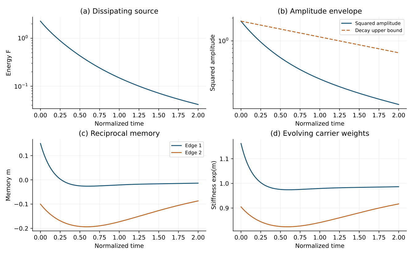
**Figure 1. The asymmetric trajectory.** Energy and squared amplitude decrease while edge memories and stiffnesses evolve differently. The amplitude envelope is the theorem's bound, without fitting. Units are those of Section 2.
The feedback difference $0.02379$ is distinct from the conditional factorization error and far larger than the $2.95\times10^{-11}$ tangent-check error. The saved collective-mode error is $2.83\times10^{-16}$. The norm of $U$ agrees with $e^{-0.48}$ and is insensitive to the adapting contrasts.
### 6.2 Pulse ordering and the symmetric control
$$
K_1=\operatorname{diag}(1,2),\qquad K_2=\begin{pmatrix}2&1\\1&2\end{pmatrix},\qquad\gamma=0.7,\quad\alpha=1.1.\tag{54}
$$
Both are positive and $\|[K_2,K_1]\|=1$. For $N=X-(\operatorname{tr}X)I/2$ and $d^2=-\det N$, $N^2=d^2I$ yields an independent $2\times2$ exponential:
$$
e^X=e^{\operatorname{tr}X/2}\left(\cosh d\,I+\frac{\sinh d}{d}N\right).\tag{55}
$$
Use the continuous value at $d=0$. The largest difference from the matrix-exponential implementation is $3.34\times10^{-16}$. The analytic bound uses individual $\tau$, not total $2\tau$.
**Table 2. Two-pulse propagation.** The final column is the relative discrepancy of the scaled matrix in (24) from its leading commutator.
| $\tau$ | $\lVert U-DV\rVert$ | Bound | Leading discrepancy |
| ---: | ---: | ---: | ---: |
| 0.04 | $1.148\times10^{-3}$ | $1.232\times10^{-3}$ | 0.19671 |
| 0.02 | $2.974\times10^{-4}$ | $3.080\times10^{-4}$ | 0.10122 |
| 0.01 | $7.566\times10^{-5}$ | $7.700\times10^{-5}$ | 0.05134 |
| 0.005 | $1.908\times10^{-5}$ | $1.925\times10^{-5}$ | 0.02585 |
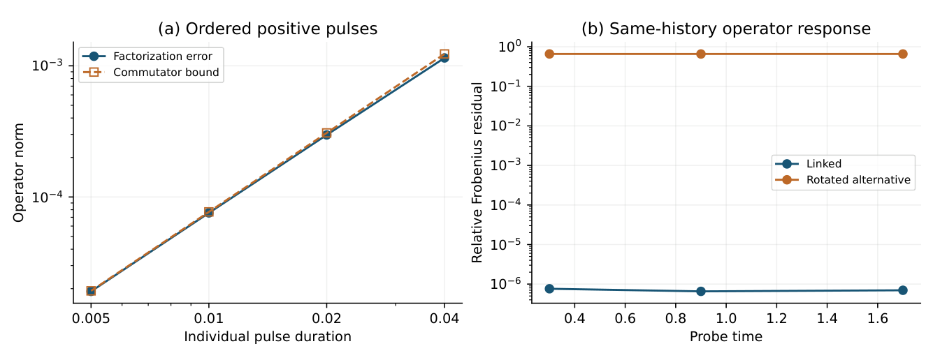
**Figure 2. Ordering and response.** Left: factorization error and commutator bound against individual pulse duration. Right: $\|\widetilde C-2\widetilde H\|_F/\|\widetilde C\|_F$ along the same recorded memory history for the linked and coherent-eigenvector-rotated responses. Connecting lines are not statistical uncertainties.
For the symmetric source control replace $z_0$ by $(1+0.2i,-0.4+0.7i,1+0.2i)^\top$ and $m_0$ by $(0.15,0.15)^\top$, retaining parameters and duration. Maximum memory displacement is $0.202353$, with $m_1-m_2$ numerically zero. Factorization residual is $4.34\times10^{-13}$, versus $0.007322$ asymmetrically. The asymmetric trapezoidal commutator diagnostic $0.0903793$ approximates the bound's integral; it is not a certified upper enclosure.
### 6.3 Response reconstruction and exact fixtures
Use times $0.3,0.9,1.7$ and $h=5\times10^{-4}$. A cubic spline through the 401 memory samples defines both replayed histories. DOP853 uses relative tolerance $10^{-12}$, absolute tolerance $10^{-14}$. Spline mismatch in hardware would belong to drift and reconstruction budgets. Rotate with the cyclic permutation
$$
S=\begin{pmatrix}0&1&0\\0&0&1\\1&0&0\end{pmatrix}.\tag{56}
$$
**Table 3. Same-history reconstruction.** The residual uses stipulated $r=2$; the fitted ratio is diagnostic.
| Time | Model | Relative residual | Fitted ratio |
| ---: | --- | ---: | ---: |
| 0.3 | Linked | $7.630\times10^{-7}$ | 1.9999986 |
| 0.3 | Rotated | $6.590\times10^{-1}$ | 1.5656839 |
| 0.9 | Linked | $6.558\times10^{-7}$ | 1.9999988 |
| 0.9 | Rotated | $6.572\times10^{-1}$ | 1.5681140 |
| 1.7 | Linked | $6.982\times10^{-7}$ | 1.9999987 |
| 1.7 | Rotated | $6.578\times10^{-1}$ | 1.5672790 |
Linked residuals below $8\times10^{-7}$ separate from alternative residuals above $0.65$ despite identical coherent eigenvalue multisets. Frozen criteria are $10^{-4}$ and $0.01$, respectively. Solver tolerances are not apparatus noise.
Diagonal fixtures use $A(t)=c\operatorname{diag}(1+t,2+t/2)$, $\gamma=0.7,\alpha=1.1$, durations $0.04,0.02,0.01$, and operator perturbations of size $10^{-10}$. Exact scalar exponentials independently check extrapolation and $5\varepsilon/h$ noise amplification. A $10^{-12}$ floating allowance does not make near-saturation directed arithmetic. Rational checks cover (34)–(36); integer identities and elementary exponentials cover nonautonomous closure; (40) gives the moving-metric fixture directly.
### 6.4 Public verification and evidence classes
The public package contains seven scientific scripts, specifications, saved outputs, asset generator, dependencies, provenance, hashes, and a runner that writes into a fresh directory. Editable manuscript source is separate. With Python 3.12 and the listed dependencies, use ordinary Python (without optimization) to run `python run_all.py --output-dir ../adaptive_verified_results` from the extracted package. The output directory must be new and outside the package. Cryptographic checks preserve reference files. Discrete results, labels, table structure and acceptance definitions are exact; scientific quantities and trajectories use specified tolerances. Small solver and finite-difference residuals are tested against scientific ceilings.
The reference run used Python 3.12.14, NumPy 2.3.5 and SciPy 1.18.1. Regenerated values must match their own underlying results at printed precision while those results meet scientific criteria. Line endings are normalized. Regressions accept line-ending and admissible diagnostic changes and reject changed science, labels, structure or acceptance conditions. Analytic proofs, rational fixtures, independent DOP853/RK4/closed-form evaluations and same-environment replay establish different things. None substitutes for physical implementation, empirical validation or interval certification. The package excludes unrelated radial, image and Kerr data.
## 7 Consequences and focused extensions
One energy supplies the adaptive carrier and reciprocal feedback. Conditional contraction and unitarity persist, with the symbol fixed on the reachable range by the mobility ratio. Exact interaction-picture propagation and the commutator bound replace the generally lost one-parameter stationarity and static factorization.
The amplitude alone does not determine its velocity on all source states. Linearization makes the lost source information explicit in the initial-memory term and causal kernel. A conditional history and a free feedback probe are different experiments. Independent calibrated operator response adds information that eigenvalue fits discard: the linked law predicts common eigenspaces and scalar action in degenerate blocks, even against the eigenvalue-preserving rotated comparison.
### 7.1 Physical implementation and driven organization
A three-node network with independent mobility calibration, known metric and phase-sensitive detectors offers a direct test. Compare a repeated clamped or replayed path with an unclamped kick. The former tests the conditional law; the latter tests the kernel. Fix alternative, initialization, probe durations, drift and detector bounds in advance. The computed contrasts suggest observables and scales, not hardware feasibility or device noise.
The unforced model relaxes to $(0,0)$. An imposed amplitude force $f(t)$ contributes supplied power $\Re[(Kz)^*f]$; driven attraction, stability and response require separate analysis.
### 7.2 Continuum domains and renormalization
A continuum model needs a closed energy form, boundary conditions, nonlinear well-posedness, and evolution-family hypotheses for time-dependent domains or a common form domain. Unbounded commutators need controlled graph bounds or bounded extensions and integral convergence; crossings are not the domain obstacle. A finite functional calculus does not define an infinite determinant budget. Cutoff removal needs trace ideals or another declared determinant convention, counterterms and convergence. Renormalization, continuum universality and a shared microscopic explanation remain separate questions.
## 8 Conclusion
The aligned finite energy and mobility law retains linked instantaneous phase and attenuation as the carrier evolves. Cross-time commutators control finite propagation; initial memory and a causal kernel control free feedback. Calibrated probes distinguish a specified eigenvalue-preserving rival under explicit preparation and error bounds. These are operational conditions for recovering the linked law from source readout.
## References
1. Jeremy Rodgers. *The Canonical Spectral-Curvature Field: A Unified Operator Origin for Coherence, Dissipation, and Spectral Budgets*. 2026 preprint, issued 3 November. [DOI](https://doi.org/10.5281/zenodo.23899458).
2. Igor S. Aranson and Lorenz Kramer. The world of the complex Ginzburg–Landau equation. *Reviews of Modern Physics* 74:99–143, 2002. [DOI](https://doi.org/10.1103/RevModPhys.74.99) · [arXiv](https://arxiv.org/abs/cond-mat/0106115).
3. Tosio Kato. Integration of the equation of evolution in a Banach space. *Journal of the Mathematical Society of Japan* 5(2):208–234, 1953. [DOI](https://doi.org/10.2969/jmsj/00520208) · [Journal](https://www.jstage.jst.go.jp/article/jmath1948/5/2/5_2_208/_article/-char/en).
4. S. Blanes, F. Casas, J. A. Oteo, and J. Ros. The Magnus expansion and some of its applications. *Physics Reports* 470:151–238, 2009. [DOI](https://doi.org/10.1016/j.physrep.2008.11.001) · [arXiv](https://arxiv.org/abs/0810.5488).
5. Jeremy Rodgers. *Observable Quotients and Exact Projected Dynamics: Closure, Memory, Minimal Dynamical Completion, and Effective Field Operators*. 2026 preprint, issued 15 July. [DOI](https://doi.org/10.5281/zenodo.21371251).
6. Jeremy Rodgers. *From Source Structure to Spectral Profiles: Generation Mechanisms and Observable Readouts in the Canonical Spectral-Curvature Framework*. 2026 preprint, issued 3 November. [DOI](https://doi.org/10.5281/zenodo.23912447).
7. Jeremy Rodgers. *Cross-Domain Spectral Ratio Structure: Refined Recurrence, Robustness and Diagnostic Limits*. 2026 preprint, issued 2 November. [DOI](https://doi.org/10.5281/zenodo.23888292).
8. Jeremy Rodgers. *Source Readout Non-Equivalence: Descent and Equivariant Reconstruction Obstructions*. 2026 preprint, issued 15 July. [DOI](https://doi.org/10.5281/zenodo.21369967).